Lecture 12: Recommendations

This lecture covers recommendation systems — the last new material before the final quiz. Some key questions to keep in mind as we go through this: What is the long tail? What's the difference between collaborative filtering and content-based recommendation systems? How do offline and online testing differ for recommenders? What is the ratings matrix, and what are implicit versus explicit user ratings? What is the cold start problem? What are common offline metrics for evaluating recommender quality? And why and how do we test recommendation systems online? These are the fundamental questions that frame our discussion of recommendation systems today.

Here are the key questions we'll work through in this section on recommendation systems. What is meant by the long tail? What's the difference between collaborative filtering and content-based recommendation systems? How does offline testing differ from online testing? What exactly is a ratings matrix? What are implicit versus explicit user ratings? What is the cold start problem? What metrics do we use to evaluate recommender quality offline? And why do we need online testing at all? These questions frame the entire discussion. By the end of this section, you should be able to answer each one clearly. We'll build up from the basics — why recommendations matter, the different approaches, how to evaluate them — and then dive deeper into specific techniques in the following sections.

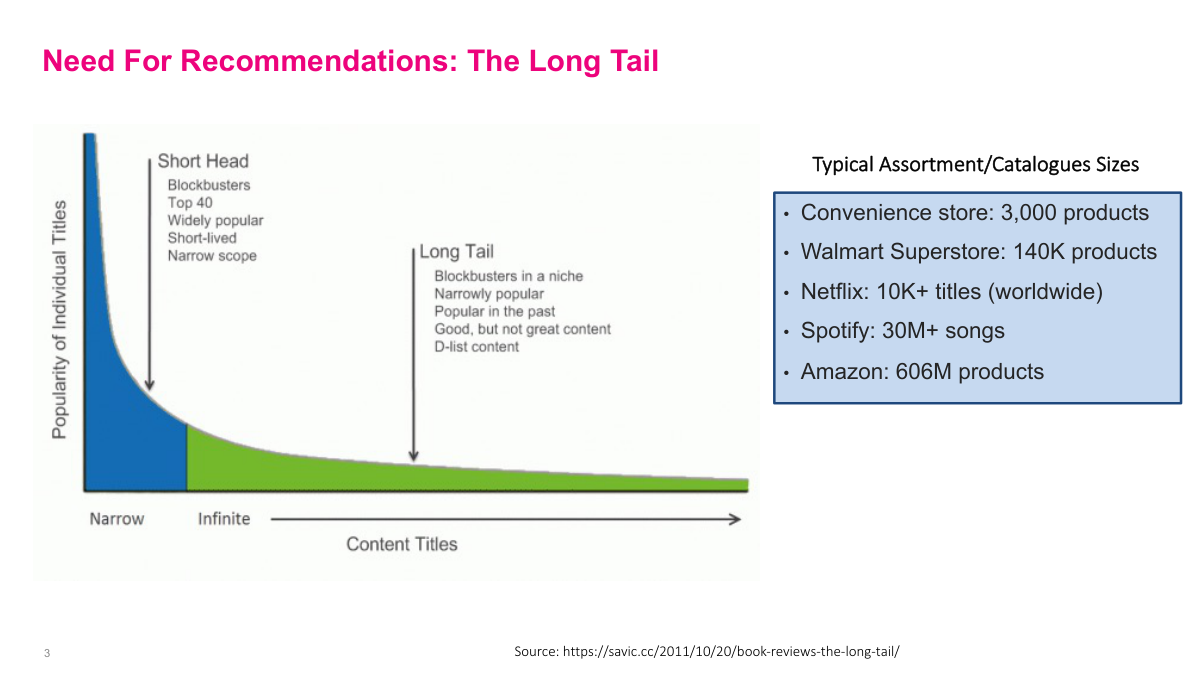
Recommendation systems have become increasingly important in the digital age. Look at the sheer volume — no single person can explore everything on Netflix, Spotify, or Amazon. These digital businesses have enormous catalogs, and they want to sell niche items too. This creates a power distribution called the long tail, where the right side of the curve holds a huge portion of total product volume. Previously, most people just bought the most popular items — you got strawberry jam because that's all the store carried. Now with the long tail, you can find something as esoteric and customized as you want, even if it's not in the top thousand products. A convenience store has three thousand products, Walmart has 140,000, Netflix has over 10,000 titles, Spotify has 30 million songs, and Amazon has over 600 million products. Recommendation systems help push this long tail, taking advantage of large catalogs. In the context of CRM and one-to-one marketing, finding the right product for a specific person is enormously valuable for the business.

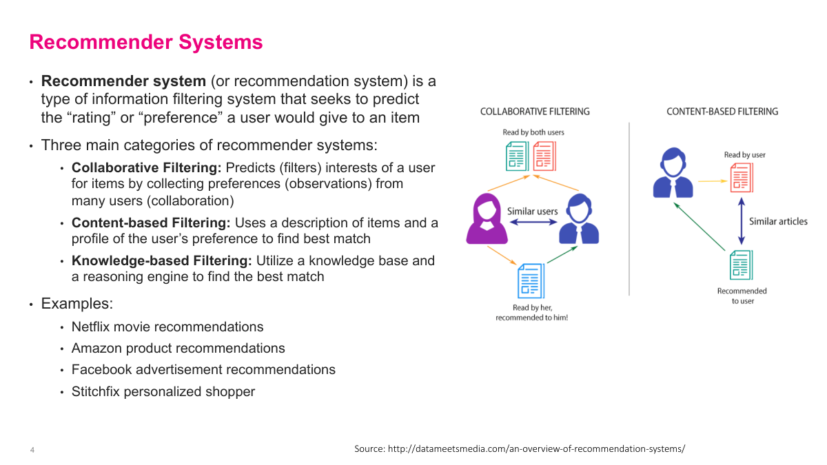
Collaborative filtering dominates at big tech companies because it leverages data from millions or hundreds of millions of users collectively. A natural question is whether you need a lot of data — and yes, platforms like Netflix and Amazon have enormous datasets. However, when data is limited, content-based filtering can actually perform well. In practice, most real systems are hybrids. While modern big tech companies primarily use collaborative filtering techniques, they also incorporate content-based filtering ideas. The combination gives you the best of both worlds — the power of collective user behavior data plus the ability to handle cases where behavioral data is sparse.

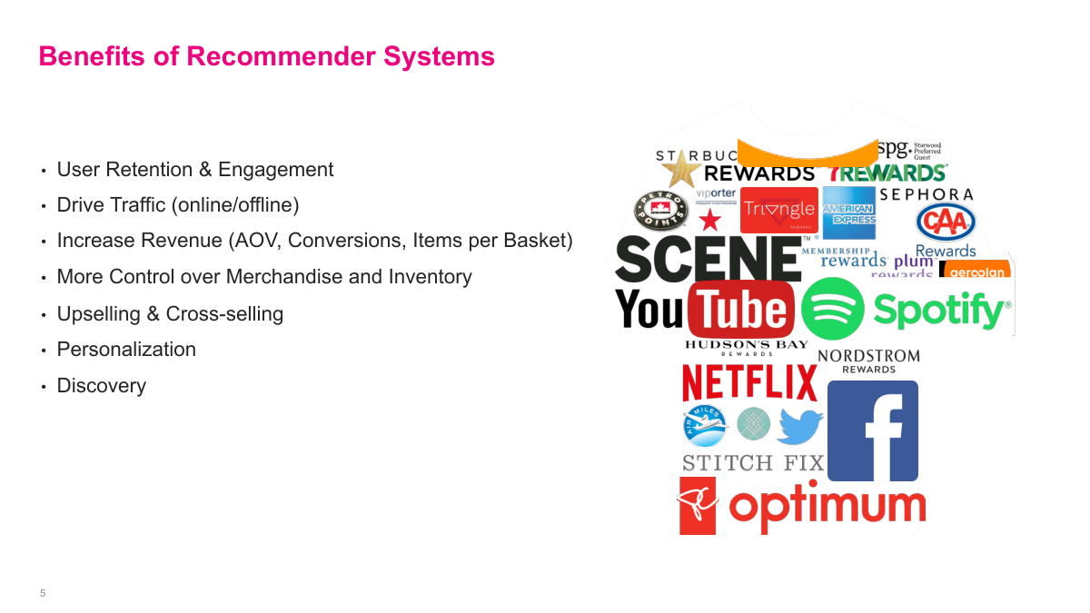
There are several benefits to recommendation systems beyond the obvious ones like user retention, engagement, and conversions — which are central to ad platforms. For more traditional businesses, there's direct revenue impact, like increasing purchase amounts. Think of Sephora recommending products to you. There are also less obvious benefits: clearing out inventory, selling discontinued items, running holiday sales, and pushing products tied to vendor deals. You can use recommendation channels to put items on sale and move them efficiently. These are all further down the hierarchy of what recommendation systems help with. But the most fundamental benefit, especially for businesses with a hundred thousand or a million-plus products, is discovery. When you don't have a physical store, helping users discover products they'd never find on their own is critical.

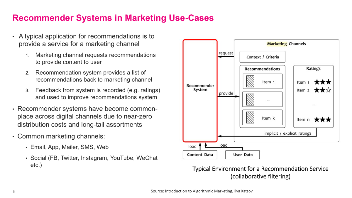
A typical abstract recommendation system starts with understanding that recommendations don't happen in a vacuum — they're pushed to a channel. That channel could be email, an app, or a display ad on a website. The marketing channel is the actual system the user interacts with. The recommendation system loads user data and content data, and when a page loads, it receives a request like: fill these three recommendation slots for this particular user. Then it serves those items. One key part is the feedback loop — when a user clicks on something or rates something, that feedback gets recorded and used to improve the recommendation system. Those observations on user behavior are critical. This is a high-level view, but the feedback loop is what makes the system improve over time.

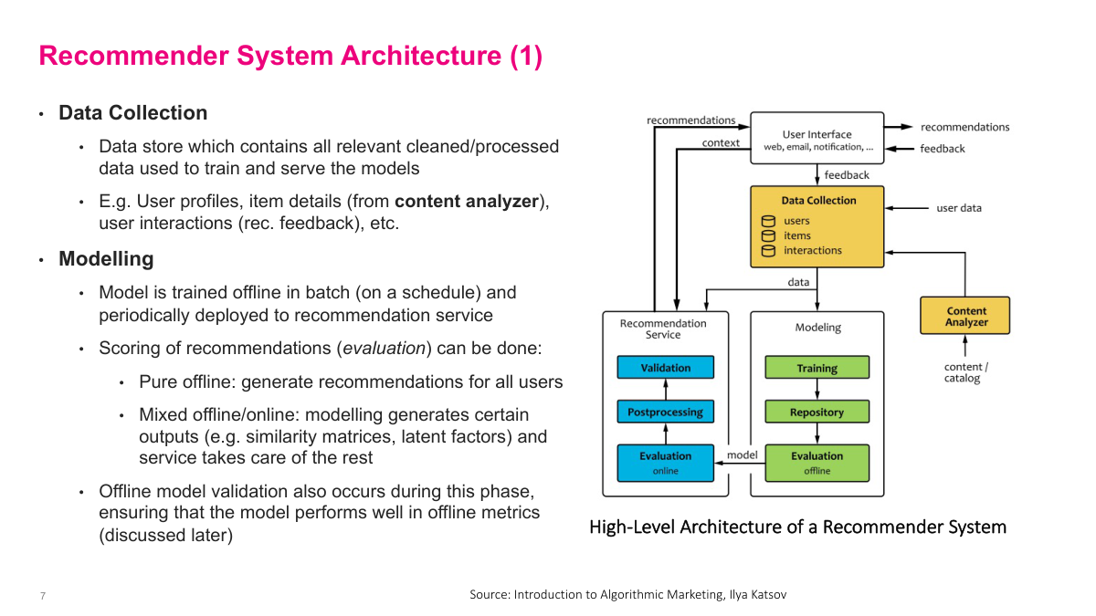
Let's step through the key components of a recommender system. First is data collection — arguably the most important part. You need a substantial database for user data, click data, and item details like product descriptions or movie catalogs, stored in a way that's usable for machine learning. Next is modeling, where you train a model, deploy it, and evaluate it offline. The critical insight here is that offline evaluation can never substitute for online evaluation. The reason is the counterfactual problem: in your historical data, you showed me five specific recommendations, but you have no way of knowing how I would have reacted to five different recommendations. You only have data from what you actually did, not from alternative actions. So while offline evaluations may correlate with real-world performance, you ultimately need online evaluation — A/B testing and similar methods — to truly measure how your recommendations perform.

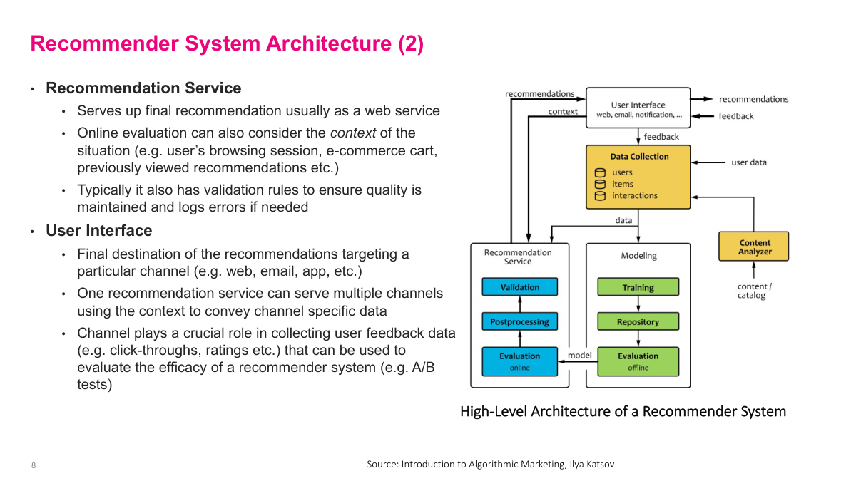
Once your model performs well in offline testing, you push it to your production recommendation service. There you typically do A/B testing and add business rules to keep the model in check. For example, if I just bought diapers yesterday, the model might recommend diapers A, B, and C because historically that's what I'm most interested in. But a simple rule can suppress that since I clearly don't need more right now. The recommendation interface calls the service saying, I have three slots to fill — what's best for this user? The service returns its top picks, which get displayed. Critically, you also need to record that feedback — what was shown, what was clicked, what was ignored — back into your data pipeline. That feedback loop is how you improve the model over time. These components might sound abstract now, but in practice you'll see concrete instances of each one. The architecture varies by company, but these building blocks — offline training, production service, business rules, and feedback logging — are universal.

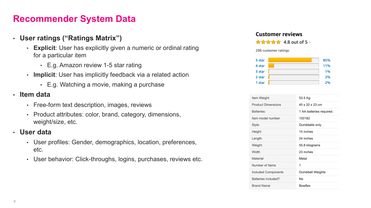
The fundamental data sources for recommender systems are the user ratings matrix, item data, and user data. The ratings matrix is the most intuitive — for each user, what have they interacted with and how much did they like it? Think Amazon reviews: user X rated product Y four out of five stars. You collect all these entries across all users and that's your ratings matrix. Sometimes ratings are explicit like star reviews, but often they're implicit. Netflix probably uses how much of a video you actually watched — if you watched an hour, that signals interest even though you never explicitly rated it. Item data is your catalog metadata: movie descriptions, directors, actors, product ingredients, and so on. User data includes whatever profile information people provide at signup plus their behavioral history — what they've clicked, watched, or purchased. These three data sources get used to varying degrees depending on the method. Some approaches rely heavily on the ratings matrix, others leverage item or user features more. We'll see how different methods draw on these sources as we go through the material.

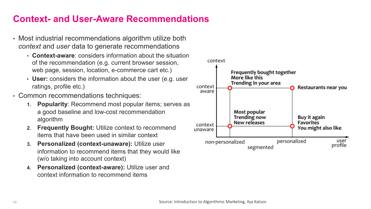
Recommendations don't necessarily have to be personalized to you specifically. You can think about this along two axes: whether the recommendation is personalized versus generic, and whether it's context-aware versus context-free. In the non-personalized, context-aware quadrant — say you're on an Amazon product page but not logged in — the system can still recommend items similar to what you're viewing. Non-personalized and context-free is like a billboard or the Netflix homepage just promoting popular movies. On the personalized, context-aware side, think of a restaurant app that knows you're a young professional and suggests places accordingly. Personalized but context-free might be Amazon's homepage showing general recommendations based on your history. If you're just starting out building a system, don't jump straight to complex deep learning models. Simple approaches work surprisingly well. The classic one is just showing the top ten most popular products — that's what retailers did for fifty years and it serves a large chunk of users well. Another easy approach is co-occurrence statistics: if someone buys product A, what do they most frequently buy alongside it?

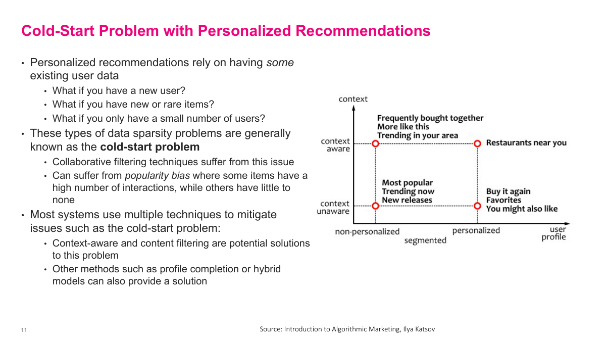
The cold start problem is a fundamental challenge in recommender systems. There are several situations where you simply don't have enough data: a new user with no history so you don't know their preferences, a new or rare item entering your catalog with no interaction data, or a new business with very few users overall. These are all cold start problems — you're starting cold. Collaborative filtering, which relies on collective user behavior, breaks down when that collective data is missing or sparse. Without sufficient data, you also suffer from popularity bias — the system defaults to recommending popular items because it lacks data on the long tail of niche products. Most production systems handle this with hybrid approaches. They primarily use collaborative filtering, but fall back to popularity-based recommendations for new users, or switch to content-based methods that leverage item features rather than user behavior. For example, if a new user shows up, just recommend the most popular items until you gather enough interaction data. Cold start is an important practical consideration — you need enough data to generate reasonable recommendations.

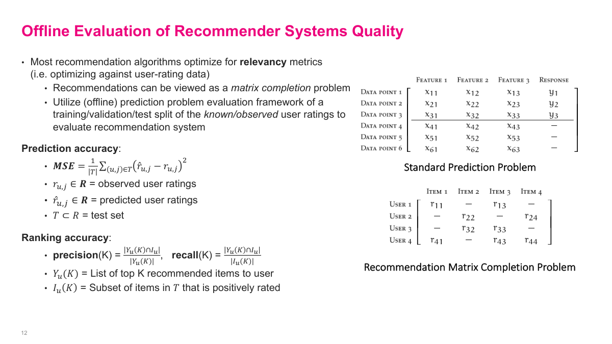
Let me explain how offline evaluation works for recommender systems. Unlike a standard supervised learning problem where you have clear training labels and predict for new examples, the ratings matrix is fundamentally different. For each user, you observe some interactions — user one bought items one, three, and five — but the missing entries aren't zeros. They're unknowns. User one might love item two but simply hasn't encountered it yet. These missing values are question marks, not negatives, and that's what makes this problem interesting. For offline evaluation, we take the observations we do have and hold out a portion — say ten or twenty percent. Then we ask: can our model accurately predict those held-out entries? The metrics we use include mean squared error for predicted ratings, and ranking accuracy metrics like precision and recall at K — of the top five items I'd recommend, how many did the user actually interact with? This simulates giving recommendations using historical data. The big limitation is counterfactuals — we can't know what would have happened if we'd actually shown different recommendations. But this approach at least ensures we're not too far off from historical behavior.

There's an important distinction between offline and online evaluation. Offline testing, which we just discussed, uses historical data to simulate recommendation quality. But the real test comes online. Typically you deploy your model to production and run A/B tests — show the new recommendations to a subset of users and compare against your existing system. Online metrics capture what offline evaluation fundamentally cannot: the actual user response to your recommendations. A model might look great on held-out historical data but perform poorly when users see and react to the recommendations in real time. That counterfactual gap is why online testing matters so much. You might find that a model with slightly worse offline metrics actually drives more engagement because it surfaces more diverse or novel items. The standard practice is to use offline evaluation as a filter — it's cheap and fast, so you screen out bad models early. Then the promising candidates go through online A/B testing where you measure real business metrics like click-through rate, conversion, and revenue. Both stages are essential to building a reliable recommendation system.

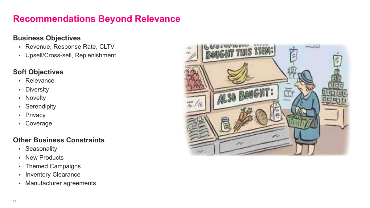
Beyond just relevance, good recommender systems need to consider several other properties. Accuracy in predicting what users want is necessary but not sufficient. Think about diversity — if I recommend five action movies and the user likes action movies, that's relevant but not very useful. Mixing in some variety gives users a better experience and helps them discover new things. Novelty matters too — recommending items the user already knows about isn't adding much value even if they're relevant. You want to surface things they haven't seen before. Serendipity goes further, recommending items the user wouldn't have found on their own that they end up loving. There's also coverage — what fraction of your catalog actually gets recommended to someone? If your system only ever surfaces the top one percent of items, that's a problem for both users and the business. And fairness is increasingly important — making sure recommendations don't systematically disadvantage certain groups of users or items. These properties often trade off against each other, so building a production system requires balancing multiple objectives, not just optimizing a single relevance metric.

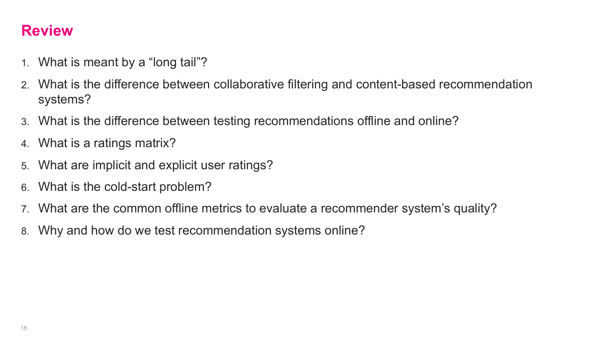
Let's do a quick review of the key concepts from this section before moving on. The long tail refers to the distribution of popularity across a product catalog — many niche products that collectively represent a huge portion of sales. Collaborative filtering uses collective user behavior data to predict what someone might like, while content-based filtering matches user profiles against item profiles. Offline testing evaluates on historical data but can never fully substitute for online testing because of the counterfactual problem — you only have data from what you actually showed users. The ratings matrix has users as rows, items as columns, and entries are either explicit ratings like star reviews or implicit signals like purchases. The cold start problem arises when you have new users, new items, or insufficient data overall. Common offline metrics include MSE for prediction accuracy and precision/recall at K for ranking quality. And you ultimately need online A/B testing to measure the real business impact of your recommendations.

Now we're moving into the second section of the lecture, which focuses on content-based filtering. This is one of the two major approaches to building recommendation systems — the other being collaborative filtering, which we'll cover in section three. Content-based filtering takes a fundamentally different approach: instead of relying on what other users have done collectively, it focuses on matching the attributes of items to the preferences of a specific user. It's more intuitive in some ways — you're directly comparing what you know about a person with what you know about a product. We'll walk through the key concepts, advantages and disadvantages, and look at concrete examples of content-based filtering algorithms.

Here are the key questions for this section on content-based filtering. What is the content-based filtering problem? What are the advantages and disadvantages of this approach? What similarity metrics can we use to compare vectors? And what is an example of a content-based filtering algorithm? These are the learning objectives we'll cover. By the end of this section, you should understand how content-based filtering works at a practical level — how to represent users and items, how to measure similarity between them, and when this approach makes sense versus collaborative filtering.

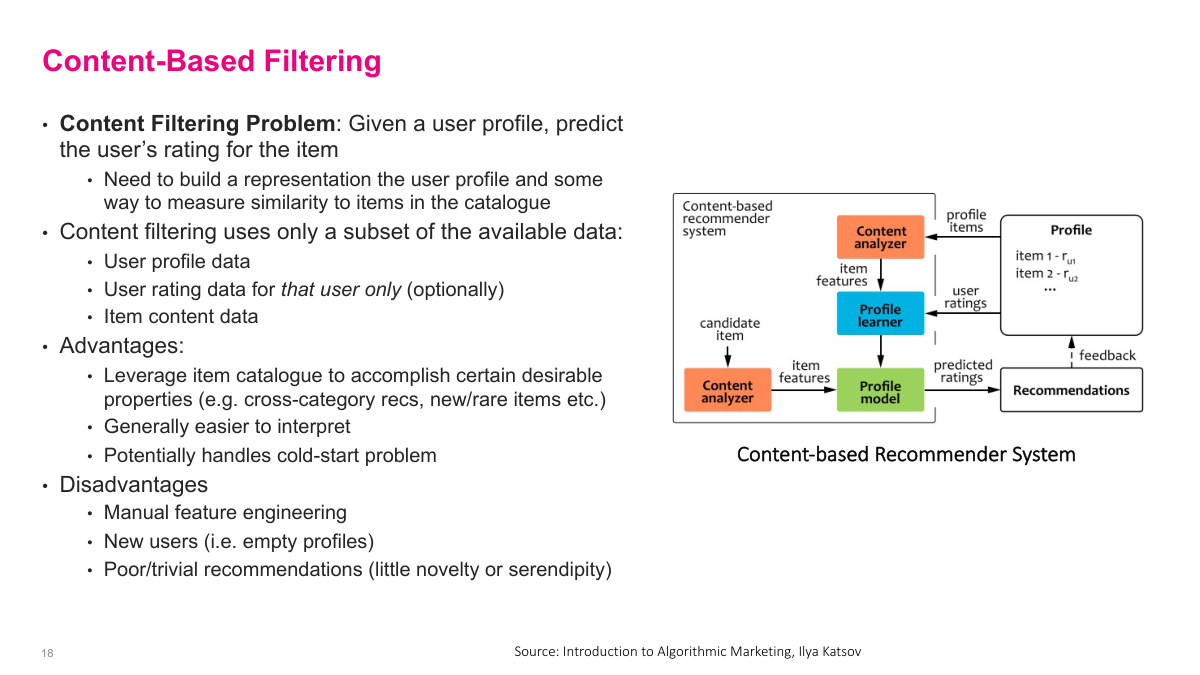
The content-based filtering problem is straightforward: given a user profile, predict that user's rating for a particular item. You need to build a representation of the user and a representation of the item, then figure out how compatible they are. Content-based filtering uses only a subset of the available data — user profile data, optionally that user's own rating history, and item content data. The advantages are significant: it leverages the item catalog, which can be very rich — think of IMDB's movie database or detailed product pages. It's generally easier to interpret, and it can handle the cold start problem because you don't need collective user data to get started. The disadvantages: it requires manual feature engineering to create good representations, new users with empty profiles remain problematic, and recommendations may lack novelty or serendipity since you're working with limited data from a single user's profile.

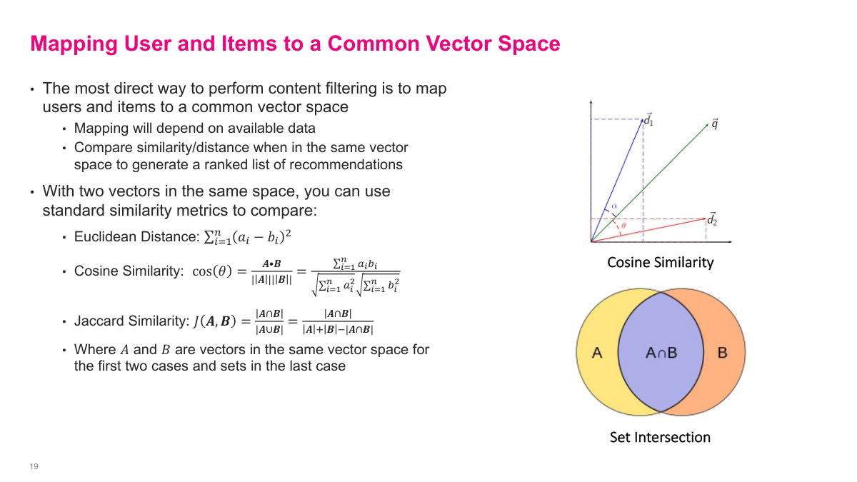
The most direct way to perform content-based filtering is to map users and items to a common vector space. If you can represent both in the same space, you can compute similarity between them — same idea as word embeddings. The mapping to this common space is the manual feature engineering you'll need to do. Once you have two vectors in the same space, there are several standard similarity metrics. Euclidean distance is the classic one, though it suffers from the curse of dimensionality. Cosine similarity measures the angle between vectors and is very popular for high-dimensional data — essentially the standard choice. Jaccard similarity is a set-based metric: you compute the intersection over the union of two sets. For example, if a user's genre preferences are comedy and romance, and an item's genres are comedy and action, the Jaccard similarity is one over three. These metrics each have their place depending on whether your data is continuous, sparse, or set-based.

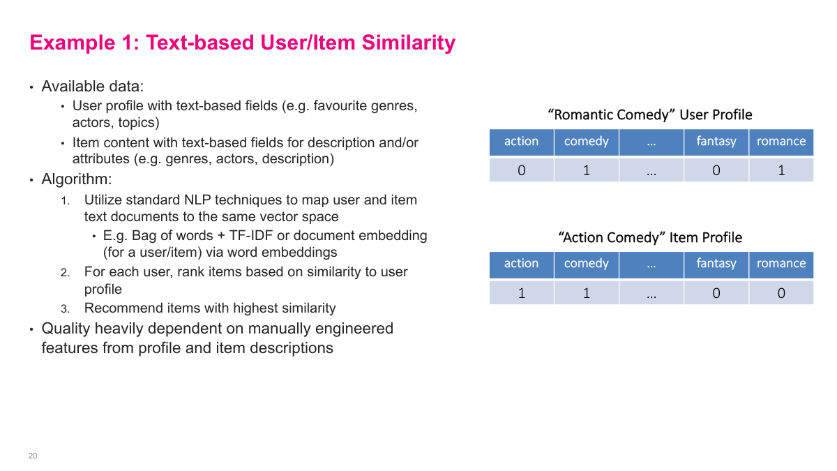
One of the simplest content-based filtering approaches is text-based user and item similarity. You have user profiles with text-based fields like favourite genres, actors, or topics, and items with similar text-based descriptions and attributes. The algorithm uses standard NLP techniques — like bag of words, TF-IDF, or document embeddings — to map both users and items into the same vector space. For each user, you compute similarities against all items and return the highest-scoring ones as recommendations. In the example here, a "romantic comedy" user profile has comedy and romance set to one, and an "action comedy" item profile has action and comedy set to one. You'd compute similarity between these vectors. The quality you get is heavily dependent on how you engineer the features — what words, categories, or discrete items you choose, and how you encode them. That said, this approach is relatively easy to implement and easy to interpret, which can be valuable in many practical situations.

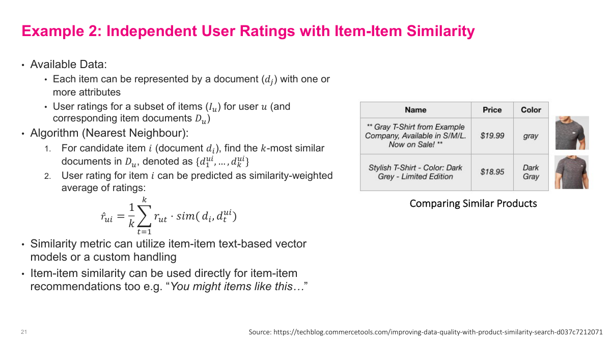
The second content-based algorithm uses item-item similarity with user ratings. Each item is represented as a document with one or more attributes, and for a given user we have their ratings for a subset of items. The algorithm works like a nearest neighbour approach: for a candidate item, find the K most similar items from the ones the user has already rated, then predict the rating as a similarity-weighted average of those existing ratings. The formula is straightforward — take one over K times the sum of the user's ratings for each similar item, weighted by the similarity between the candidate item and that rated item. The similarity metric can be text-based vector models or custom handling. This approach can also be used directly for item-item recommendations — the classic "you might like items like this" on product pages — without even needing a user profile. You're simply finding items that are similar to the one being viewed based on their attributes like product descriptions, colours, and prices.

The content-based filtering problem is: given a user profile, predict that user's rating for a particular item. You're only using data from that specific user. Implicitly, you need to build some representation of the user and some representation of the item, then figure out how compatible they are. Content-based filtering uses only a subset of the available data — the specific user's information plus item information. The advantages: it leverages the item catalog, which can be very rich. Think of IMDB's movie database or detailed product pages — that's valuable data to use. It's usually easier to interpret — you look at the user profile, look at the item, and the match is intuitive. It can also handle the cold start problem because you don't need everyone's collective data. You can find similarity between what a user has bought and even a new item. The disadvantages: manual feature engineering is required, new users with empty profiles remain problematic, and recommendations may not be great since you're working with limited data from just one user's profile.

Now we're moving into the third and final section — collaborative filtering. This is the approach that dominates at big tech companies and is the most widely used in practice. Unlike content-based filtering, which relies on item features and a single user's profile, collaborative filtering leverages the collective behaviour of all users to make predictions. The key insight is that if many users who liked items A and B also liked item C, then a new user who likes A and B will probably like C too. We'll cover the fundamentals of collaborative filtering, including neighbourhood-based methods and the more powerful latent factor models that drove innovations like the Netflix Prize.

Here are the key questions for this section on collaborative filtering. What are the advantages and disadvantages of collaborative filtering? What are rating biases and why do we need to account for them? How do neighbourhood-based collaborative filtering methods work? Can you describe a latent factor-based collaborative filtering system? What are the advantages of the latent factor approach? And what is meant by implicit feedback in collaborative filtering? These six questions cover the core concepts we'll work through. By the end of this section, you should understand both the simpler neighbourhood-based approach and the more sophisticated latent factor methods, along with practical considerations like rating bias correction and handling implicit feedback signals.

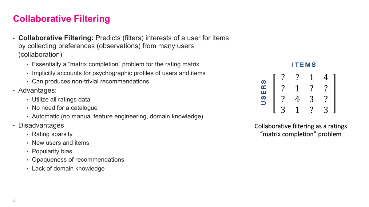
Collaborative filtering predicts a user's interests by collecting preferences from many users collectively. It's essentially a matrix completion problem — we have a ratings matrix with users as rows and items as columns, and we want to fill in the missing entries. The advantages are significant: we use all the ratings data, not just a single user's row. We don't need an item catalog or good product descriptions. And we don't need manual feature engineering — just the ratings matrix and a model pops out. It can also produce non-trivial recommendations that surprise users. The disadvantages are equally important: rating sparsity is a problem, especially for long-tail items with few interactions. There's the cold start problem with new users and items. Popularity bias means the system tends to recommend what's already popular. The models are typically black boxes with less interpretability. And we aren't leveraging any domain knowledge — it's purely a statistical approach.

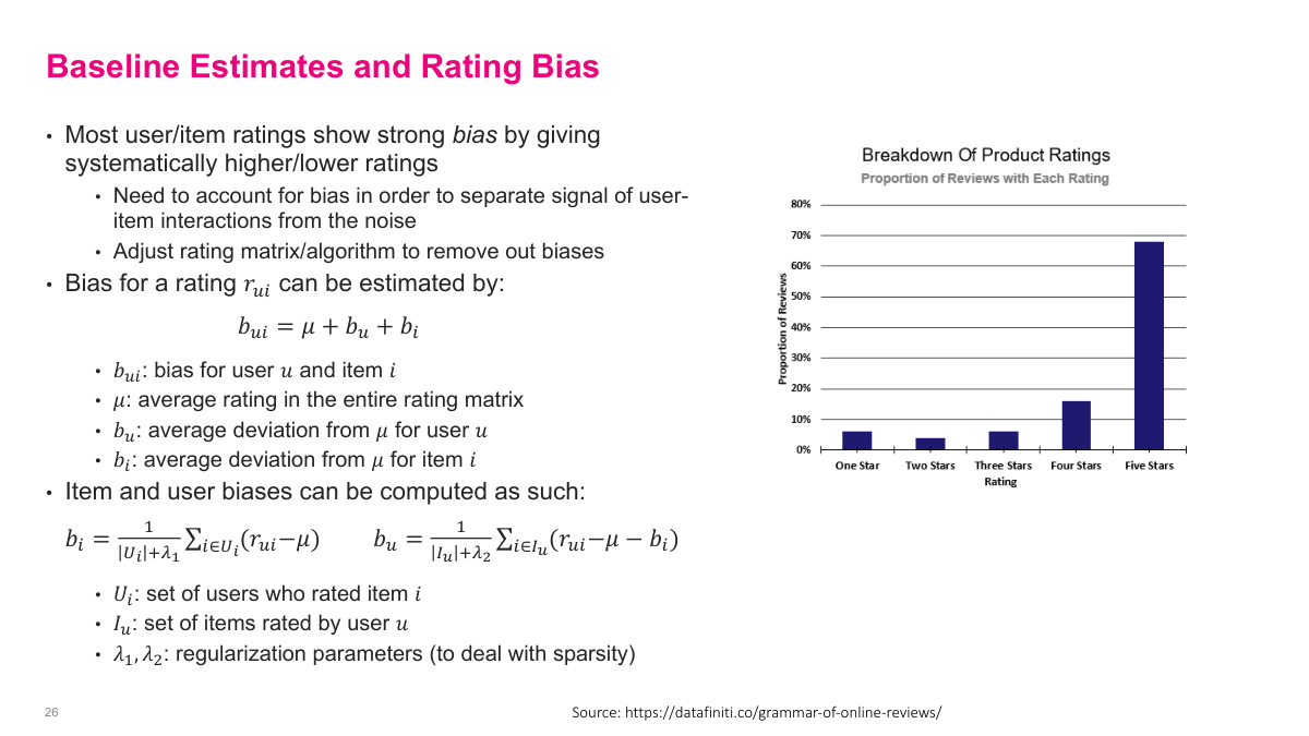
One major problem with user ratings is that they're inherently biased. Most user-item ratings show strong bias — users systematically give higher or lower ratings. When I started using Uber, I'd give a fine ride a four out of five. Then I found out most people give fives unless it's terrible. You see very skewed distributions — the chart here shows about 70% of product ratings are five stars. We need to account for these biases to separate the real signal of user-item interactions from noise. The bias for a rating can be estimated as mu (the global average rating) plus the user's average deviation from that global average, plus the item's average deviation. To compute item bias, you average that item's ratings and subtract the global mean. For user bias, you subtract the global mean and item bias from the user's ratings and average. Regularization parameters handle sparsity. This preprocessing step removes systematic biases before building collaborative filtering models and can meaningfully improve recommendation quality.

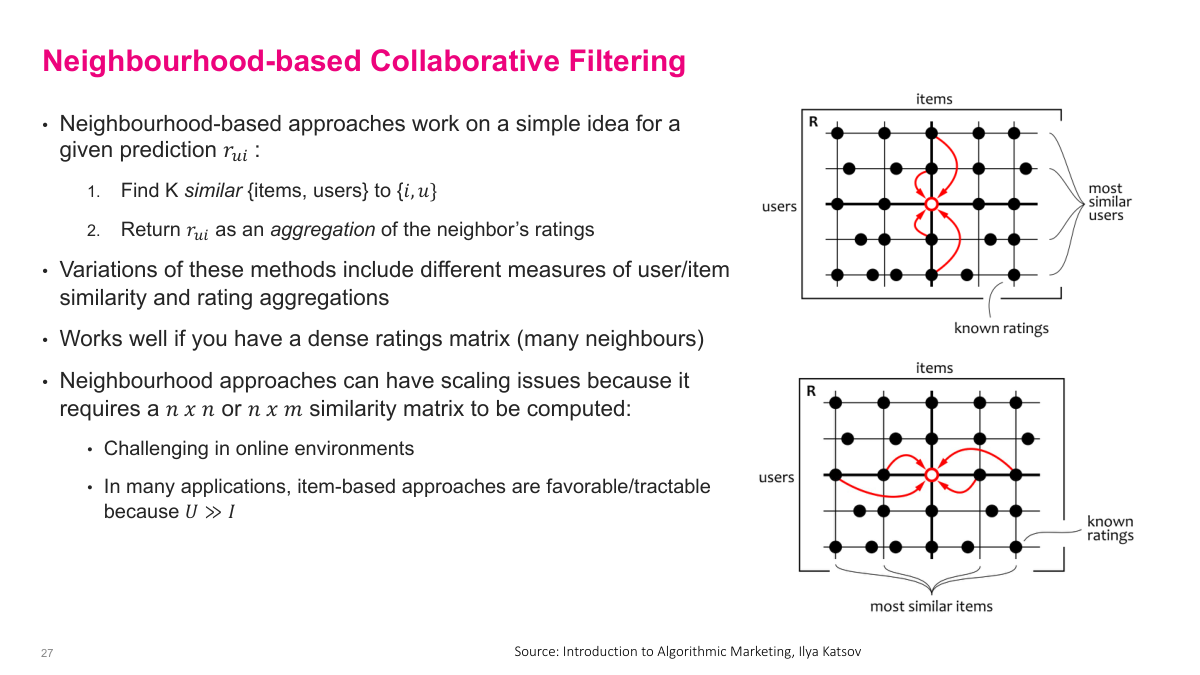
Neighbourhood-based collaborative filtering works on a simple idea: for a given prediction, find K similar items or users, then return the predicted rating as an aggregation of the neighbours' ratings. You can go along the user dimension — find similar users who rated the target item — or the item dimension — find similar items that the target user has rated. Variations of these methods differ in how they measure user or item similarity and how they aggregate ratings. This approach works well when you have a dense ratings matrix with many neighbours to draw from. But there are real scalability challenges. Computing an n-by-n or n-by-m similarity matrix is expensive. If you're doing this online with 100 million users, finding the most similar users is essentially infeasible. Items are usually more manageable — maybe 10,000 or 100,000 — which is why item-based approaches are often favourable in practice, since typically the number of users far exceeds the number of items.

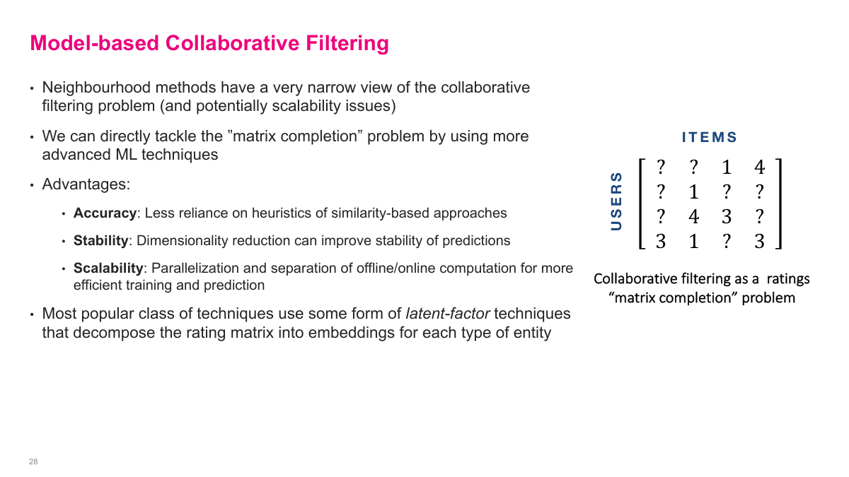
Neighbourhood methods have a very narrow view of the collaborative filtering problem and can face scalability issues. Model-based collaborative filtering takes a different approach — we can directly tackle the matrix completion problem using more advanced ML techniques. Instead of relying on local similarity heuristics, we build a model that uses the entire ratings matrix. The advantages include better accuracy since we're not relying on heuristic similarity measures, improved stability through dimensionality reduction, and better scalability since we can separate offline training from online prediction. The most popular class of model-based techniques uses latent factor methods that decompose the rating matrix into embeddings for each type of entity — users and items. These latent factor approaches form the foundation for modern collaborative filtering and are what we'll focus on next.

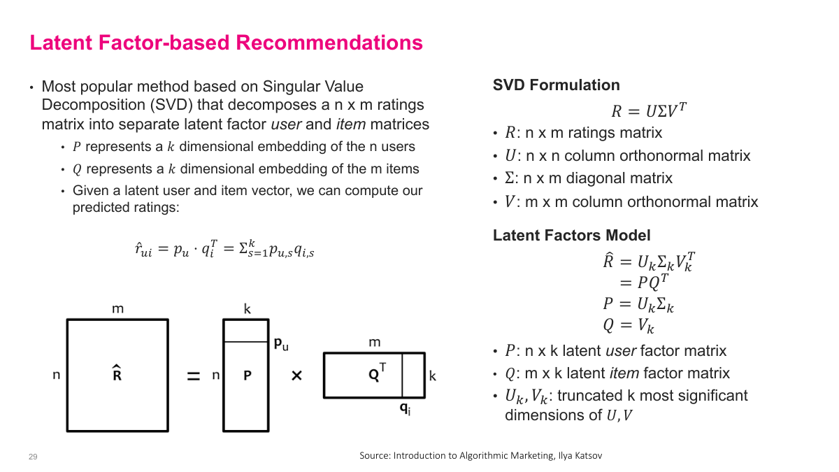
The most popular latent factor method is based on Singular Value Decomposition. You take your n-by-m ratings matrix R and decompose it into U, sigma, and V matrices. The key insight is that you can approximate this decomposition by truncating to only the top K dimensions, giving you two smaller matrices: P, which is n users by K, and Q, which is K by M items. For a particular user, their row in P is a K-dimensional dense vector representation. For an item, its column in Q is also a K-dimensional dense vector. These vectors live in the same latent space — the dot product of a user vector and an item vector approximates that user's rating for that item. This is elegant because even for user-item pairs we haven't observed, we can compute an estimate. The predicted rating is simply the dot product of the user's embedding and the item's embedding — a sum of element-wise products across the K latent dimensions.

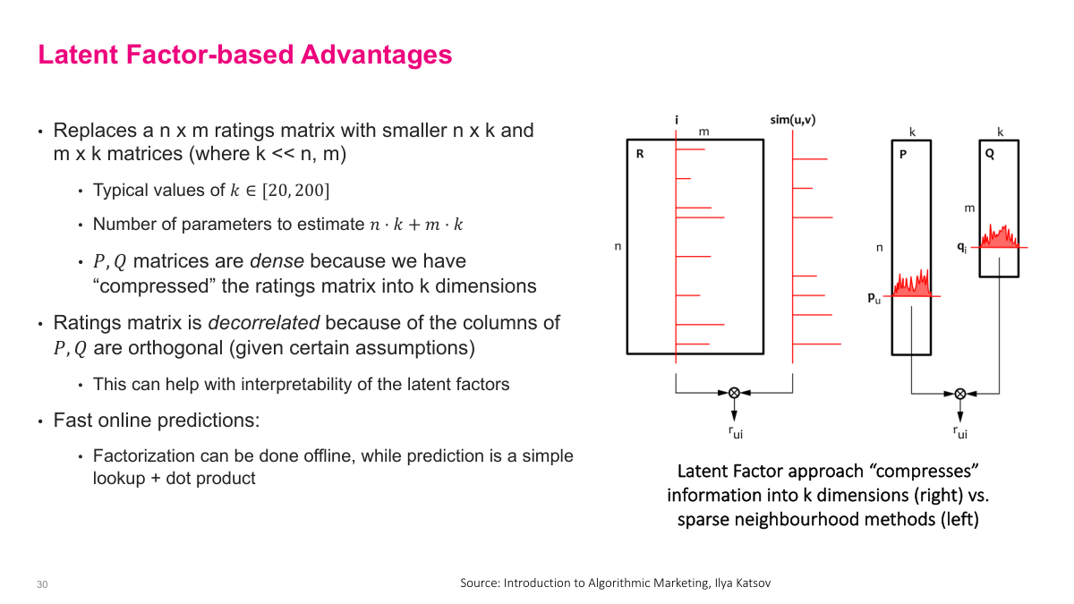
The latent factor approach has several key advantages. It replaces the large n-by-m ratings matrix with two much smaller matrices — n-by-K and m-by-K — where K is typically between 20 and 200. The number of parameters to estimate is only n times K plus m times K, which is orders of magnitude smaller than the original matrix. These P and Q matrices are dense because we've compressed the sparse ratings matrix into K dimensions. The ratings matrix is decorrelated because the columns of P and Q are orthogonal, which can help with interpretability of the latent factors. Most importantly, online predictions are extremely fast — the factorization is done offline during training, while prediction at serving time is just a simple lookup of the user and item vectors plus a dot product. This separation of offline training from online prediction makes the approach highly scalable for production systems, which is why it became so widely adopted.

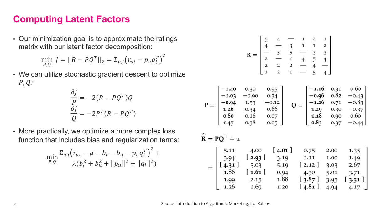
Our minimization goal is to approximate the ratings matrix with our latent factor decomposition. We minimize the squared Frobenius norm of the difference between R and P times Q transpose, which is the sum of squared errors between observed ratings and our predicted ratings. We can use stochastic gradient descent to optimize P and Q, with gradients that are straightforward to compute. In practice, we optimize a more complex loss function that includes bias terms and regularization. The full loss subtracts the global mean mu, the user bias, and item bias before computing the error from the dot product of user and item vectors. Regularization terms on the biases and the embedding vectors prevent overfitting. The example on this slide shows a concrete ratings matrix R being decomposed into P and Q matrices with K equals three, and the resulting approximation R-hat equals P times Q transpose plus mu. The bracketed values in the approximation are the predicted ratings for entries that were missing in the original matrix — that's the matrix completion in action.

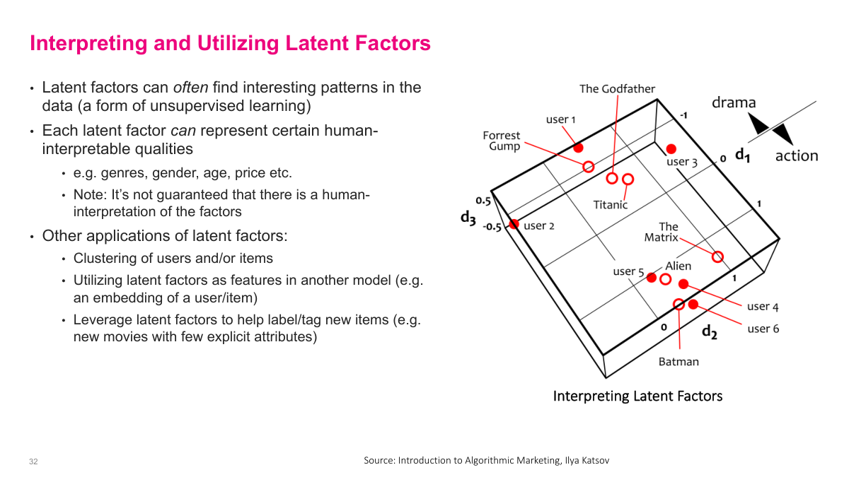
Latent factors can often find interesting patterns in the data — it's a form of unsupervised learning. Each latent factor can represent certain human-interpretable qualities like genres, gender, age, or price sensitivity, though it's not guaranteed that there will be a clear human interpretation for every factor. The 3D visualization here shows movies like The Godfather, Forrest Gump, Titanic, The Matrix, Alien, and Batman positioned along three latent dimensions — one that might correspond to drama versus action, and others capturing different taste dimensions. Users are positioned in the same space based on their preferences. Beyond recommendations, latent factors have other useful applications: clustering users and items into natural groups, using the latent factor vectors as features in other downstream models — essentially as user or item embeddings — and leveraging latent factors to help label or tag new items that have few explicit attributes.

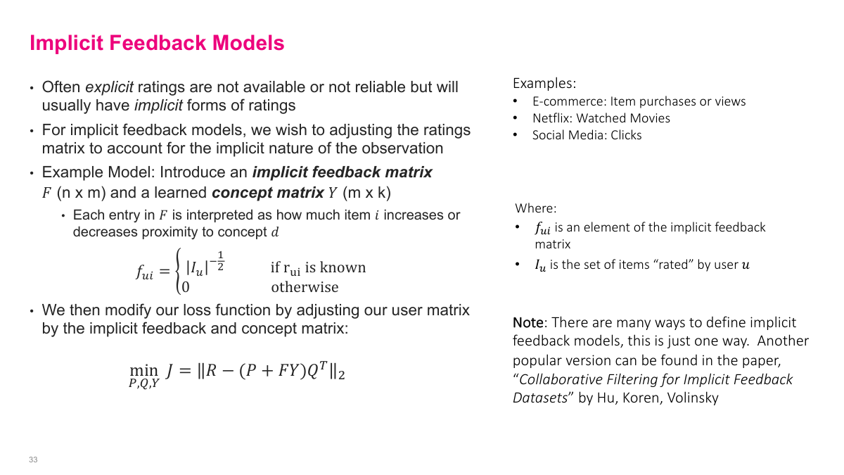
Often explicit ratings are not available or not reliable, but we usually have implicit forms of ratings — e-commerce purchases or views, Netflix watch history, social media clicks. For implicit feedback models, we want to adjust the ratings matrix to account for the implicit nature of the observations. One approach introduces an implicit feedback matrix F and a learned concept matrix Y. Each entry in F is interpreted as how much item i increases or decreases proximity to concept d. The feedback matrix entry is set to the inverse square root of the number of items the user has rated if the rating is known, and zero otherwise. We then modify our loss function by adjusting the user matrix — instead of just P, we use P plus F times Y, and multiply by Q transpose. This incorporates the implicit feedback signals into the latent factor model. There are many ways to define implicit feedback models — the paper "Collaborative Filtering for Implicit Feedback Datasets" by Hu, Koren, and Volinsky presents another popular approach.

Let's review the key questions from this section on collaborative filtering. What are the advantages and disadvantages? CF uses all the ratings data without needing item catalogs or manual feature engineering, but faces challenges with sparsity, cold start, and popularity bias. What are rating biases? Users have systematic tendencies — some rate everything high, some low — and we correct for global, user, and item biases using averaging formulas. How do neighbourhood-based methods work? Find similar users or items, aggregate their ratings — simple but with major scalability challenges. What is latent factor-based CF? Decompose the ratings matrix into two lower-dimensional matrices using SVD, giving dense vector embeddings for users and items in a shared K-dimensional space. The advantages include using the full matrix, scalability via separated offline/online computation, and no need for heuristics. Finally, implicit feedback refers to signals like purchases, clicks, and views rather than explicit star ratings, and we can incorporate these into the latent factor model through modified loss functions.