Lecture 04: Tuning

In this section, I'll clarify some of the main ideas about capacity, overfitting, and underfitting in neural networks. These are fundamental concepts you need to understand as we move beyond just optimization into the broader challenges of machine learning.

Here are the key questions you should be able to answer after this section: What are the two main challenges in machine learning? What is training, testing, and generalization? What are training, testing, and generalization gaps? What is meant by overfitting and underfitting? What is model capacity? What is the difference between training, validation, and test sets? Describe the modern approach to fitting models. Pay attention to these concepts as they're fundamental to everything we'll discuss.

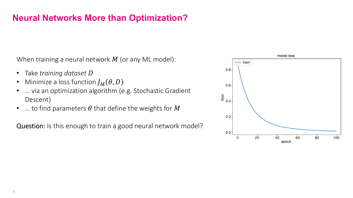
We've spent considerable time on stochastic gradient descent — understanding why it works, how it works, and building intuition around it. We have neural network models with many parameters, training datasets, and we minimize loss functions with SGD to find the right weights. But why isn't this good enough? What's the problem with just doing that? The model has to generalize to unseen data. That's exactly right. We can train successfully on training data, but what about other data points? This is the overfitting problem I've mentioned — especially when you use more layers and parameters than needed, there's a high risk of overfitting. Generalization is the key challenge.

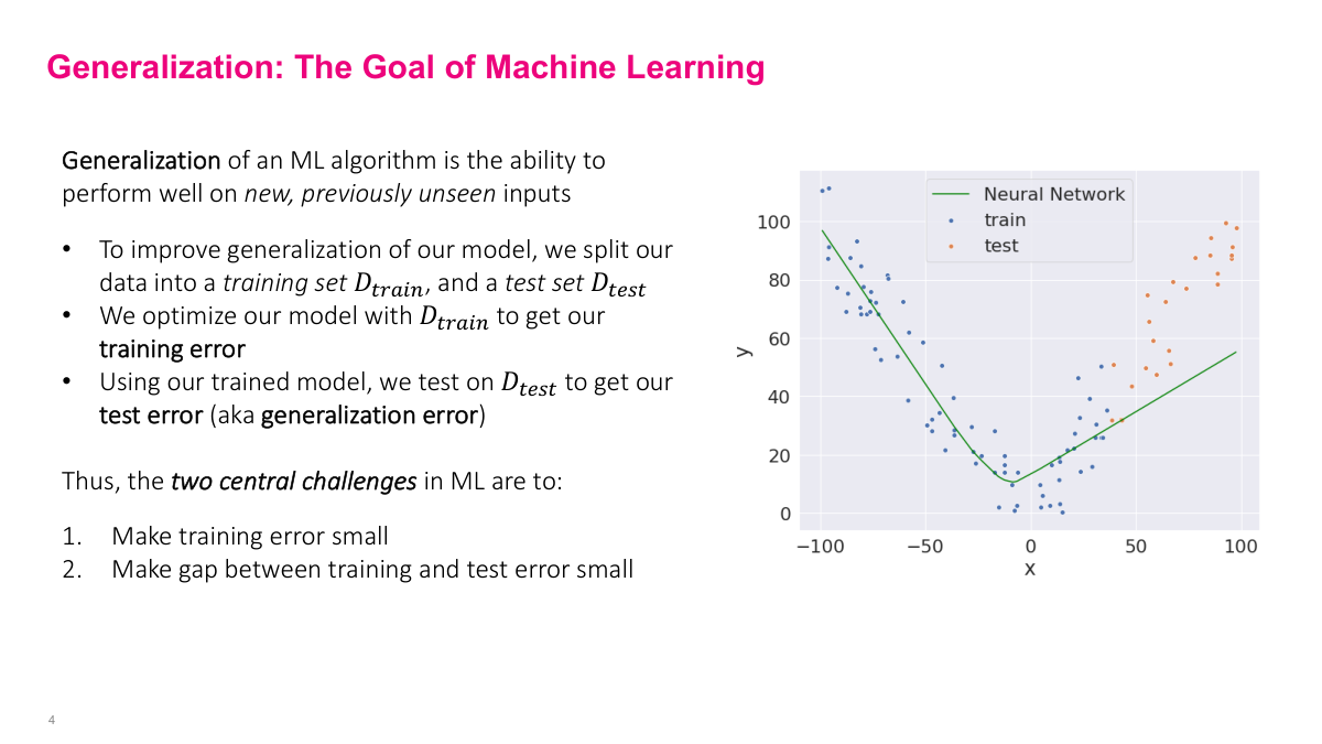
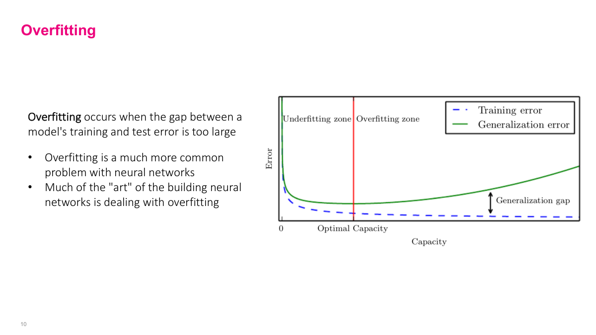
We're training on the training dataset and minimizing loss there, but that doesn't necessarily say anything about other data points — particularly ones we'll see in the future, or even your test dataset. What we really want is to minimize training error so we can model the problem well, but also ensure the testing error isn't far from the training error. The gap between training and testing error — the generalization error — shouldn't be too big. We want our model to perform well on data we've never seen before. The two main challenges in machine learning are: getting a model that can reduce training error very low (modeling the problem well), and ensuring it generalizes well by keeping the gap between training and test error small.

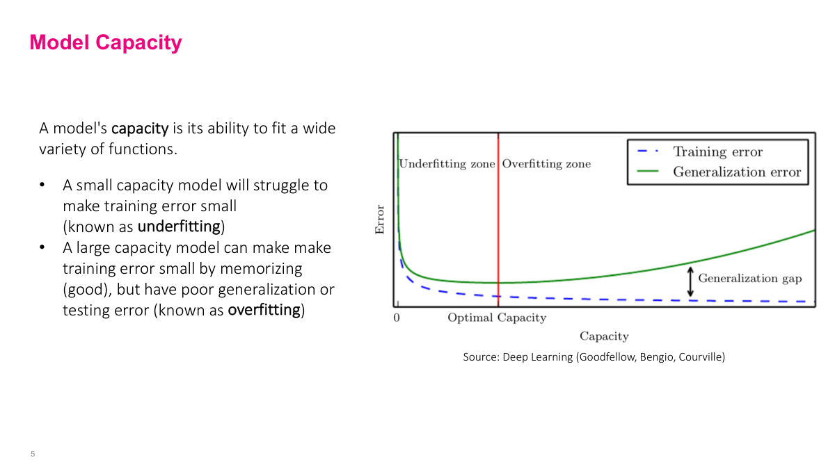
Capacity isn't a mathematical formula but a general concept — a model's ability to model different patterns. More capacity means the model can handle and model more complex functions. Adding more layers, more neurons per layer, more parameters increases capacity. But as you increase capacity, what happens? Our chance for overfitting increases. Training error definitely goes down and probably hits a plateau, but the model starts learning noise in the data, not the actual signal. When it learns noise rather than real signals, it gets more error when trying to generalize to unseen data. The green line grows — generalization error grows. This is a bigger problem with higher capacity models. But one benefit of neural networks is that we have very high capacity models, so we need to figure out how to deal with this. The traditional approach would find "optimal capacity" but that's not what we'll do.

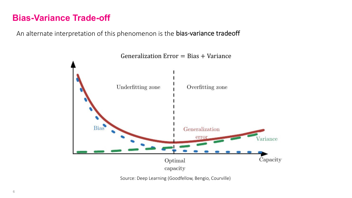
This is a more statistical explanation, but it's basically the same thing. As you increase capacity with bigger, more complex models, you start modeling the variance in the data — the noise — instead of modeling or lowering the error from the actual truth signal, which is the bias. This is another view of the capacity versus overfitting problem.

In neural networks, it's super easy to change model capacity. You can choose different model types — simple linear functions have limited capacity, neural networks have enormous capacity, tree-based models have varying capacity. Since we're focused on neural networks, we can change the hyperparameters (architecture) to increase capacity: number of hidden layers, width of each hidden layer, and other related hyperparameters. That increases capacity and probably reduces training error. But how do we ensure generalization? There are different ways: modifying learning algorithm hyperparameters, adding more data (always good), and the main way we'll discuss — regularization. That's how we actually avoid overfitting.

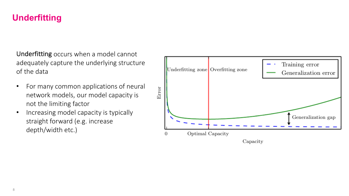
Underfitting is when your model isn't complicated enough — doesn't have high enough capacity to model the actual patterns in the data. This usually isn't the main problem in neural networks because we have so much capacity. In other types of models, especially linear models, this can be a big problem. We won't spend much time on underfitting since it's not typically our main concern with neural networks.

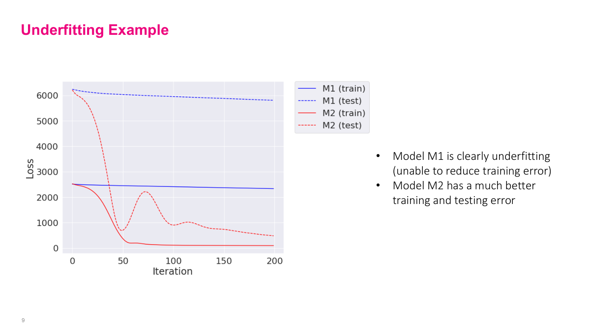
The solid line is training and the dotted line is test. You can see that the training error is very high — basically not improving the loss much. This indicates your model is underfitting. If training error is high, testing error will correspondingly be high. This contrasts with the M2 model where training error drops down nicely and testing error, though a bit volatile, settles to something not much higher than training error. Generally, these plots help you understand if you're overfitting or underfitting. Look at training error, then testing error. For model choice, I'd still choose 200 iterations to minimize testing error. Underfitting generally isn't a problem — if you see it, just increase layers, increase training time. There are many levers to avoid underfitting.

Overfitting is a much bigger problem because we have huge capacity. It's somewhat of an art to figure out how to make sure the generalization gap isn't very big. We'll pick high capacity models but use techniques, particularly regularization, to minimize this gap. It's an art to figure that out.

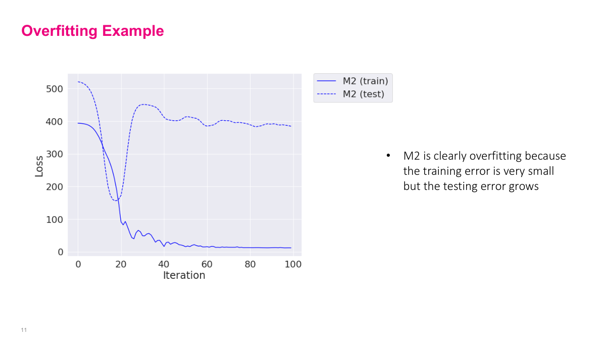
A more common thing you'll see in neural networks is training error dropping down a lot (solid blue line), but testing error jumping up. This gap indicates overfitting, especially if you see this dip and then pop up. Very likely your neural network is learning noise instead of signal. Depending on the situation, you might take the checkpoint from the earlier point and use those parameters, or add regularization and other techniques to make both curves look better. It depends on the situation.

In machine learning, one of the biggest challenges — why it's an art — is picking your hyperparameters: number of layers, width, learning rate, batch size, all those things. Most of the methodology is living and dying by your validation set. We want the validation set to be representative, then use it to make decisions about hyperparameters. Train to ensure loss decreases, but watch your validation set to ensure it's also decreasing. If not, go back and change your architecture or hyperparameters to make the validation error go down. Use a holdout test set that you don't use for hyperparameter decisions — that's your final check to ensure you're actually generalizing properly. These sets are proxies for the actual generalization error on unseen data, so you want good, representative datasets and proper separation.

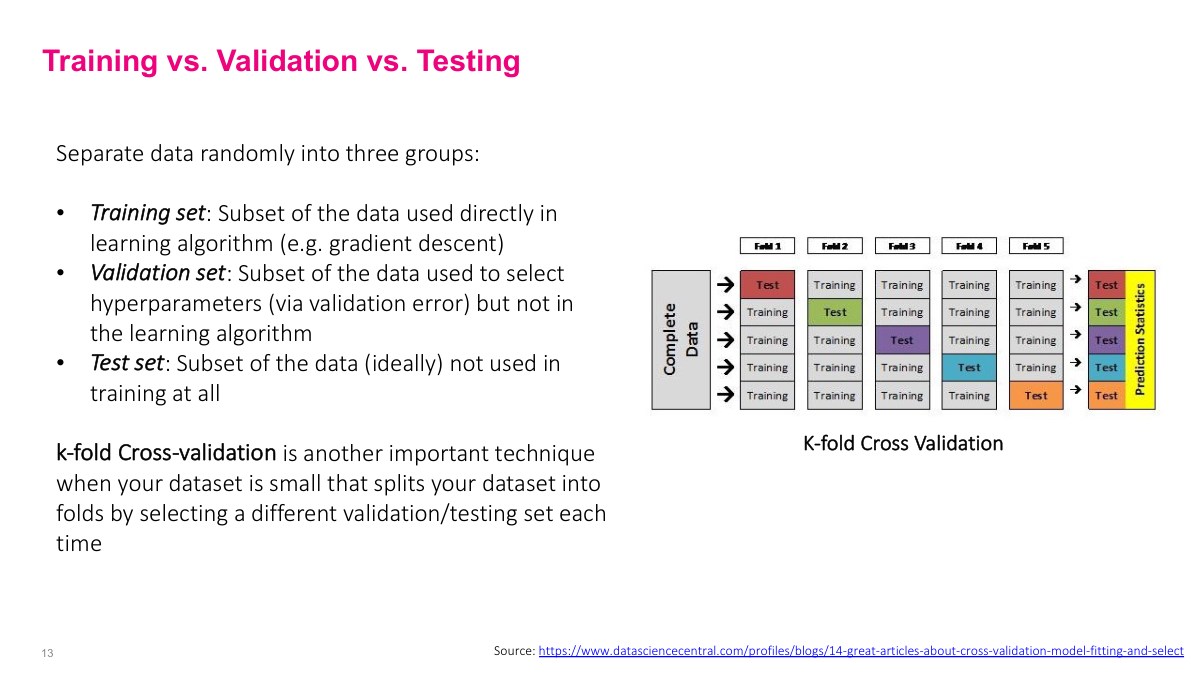
You can use k-fold cross-validation as well, depending on how much data and compute you have. Instead of just having a single validation set, cross-validation can give you more robust estimates of model performance.

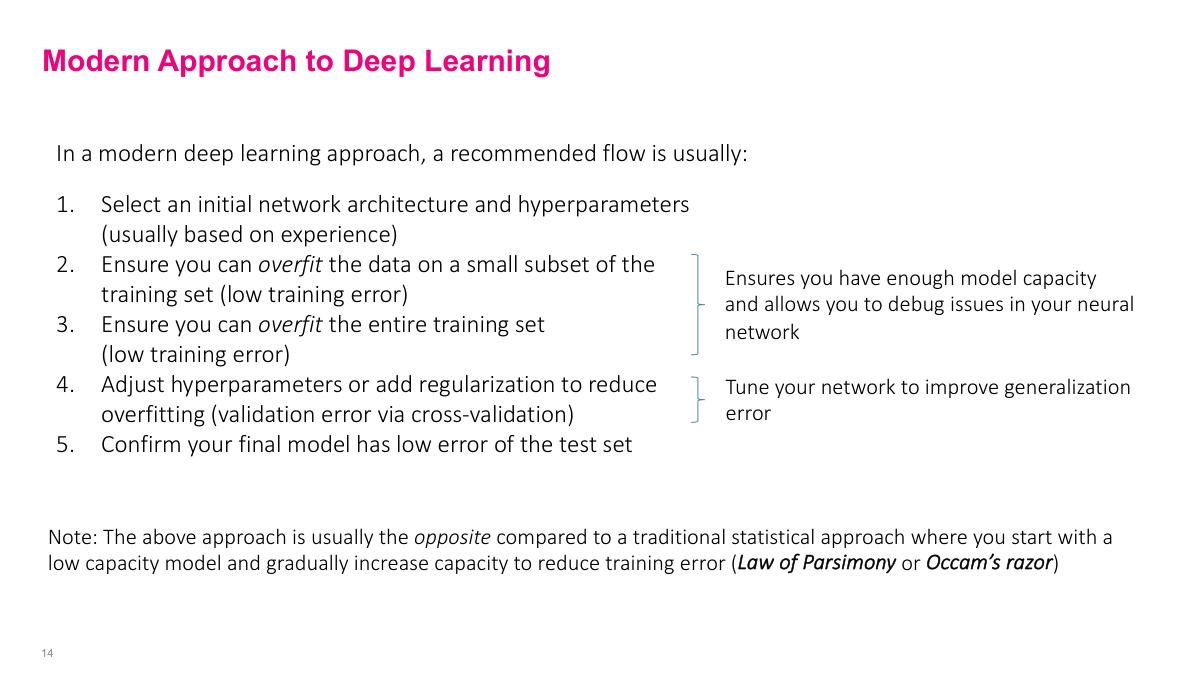
This is the modern approach to deep learning, probably different from how you've thought about machine learning before. First, pick some reasonable initial neural network architecture based on experience and guidelines. Take a small portion of your training set and try to overfit on that small portion. This serves multiple purposes: small data means fast iteration, it helps you debug errors early when it's cheap, and ensures you don't have bugs. Third, increase to the full training set size and ensure you can still overfit. This confirms you have enough capacity to model the problem. Steps one through three get you to a place where you're sure you don't have bugs and have enough capacity. Then look at generalization error (validation error) and tune your network to get a low training-validation gap by changing hyperparameters or adding regularization. You'll spend most time in step four. Finally, use your test set to confirm you had the right choices. This is different from classical approaches that start with low capacity and increase until finding optimal capacity. We don't care how the model works underneath — we just want good prediction.

Let me review the key concepts. Why is just training a neural network not good enough to guarantee a good model? It will overfit on the data and not generalize well — we're not thinking about generalization at all. What are the two main challenges? Minimize training error so the model can actually model the patterns in the training data, and make sure the generalization gap or generalization error is low. What is training and testing error and the generalization gap? Training error is error on the training set, testing error is error on the testing set (which should represent generalization if constructed properly), and generalization gap is the difference between those two. What is overfitting and underfitting? Underfitting means you can't minimize training error — your model doesn't have enough capacity. Overfitting means training error is small but the gap between training and testing error is huge — you're learning noise, not signal. What is model capacity? How complex a data distribution you can model, generally related to hyperparameters like depth and width. What's the difference between training, validation, and test sets? Training trains the model, validation is used to select hyperparameters by looking at metrics, test is used to verify the model truly generalizes without being used in modeling decisions. The modern approach: select architecture, work with a subset to debug and ensure capacity, scale to full training set, tune hyperparameters and add regularization, then test on holdout data.

Regularization is something you probably didn't have to think about explicitly in other types of models. This is the second biggest part of deep learning. I want to get across several different concepts today.

What is regularization? What are norm penalties? What is data augmentation? What is bagging? What is dropout? And what's the ideal type of regularization?

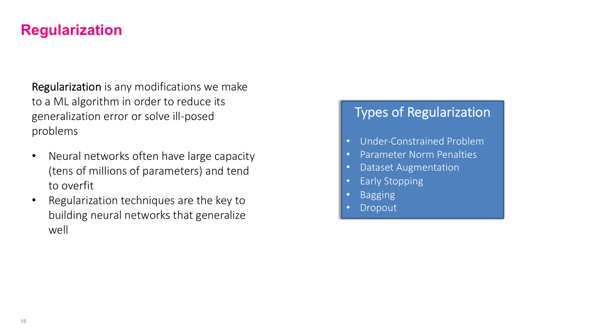
Regularization is a general concept — basically any modification we make to a machine learning algorithm to reduce the generalization error or, in more minor cases, solve ill-posed problems. Neural networks have large capacity — tens of millions or billions of parameters — and often overfit. So we really need regularization to ensure generalization error gets small so the model can actually be useful and predict new things. Regularization is a general set of techniques we can use to reduce generalization error.

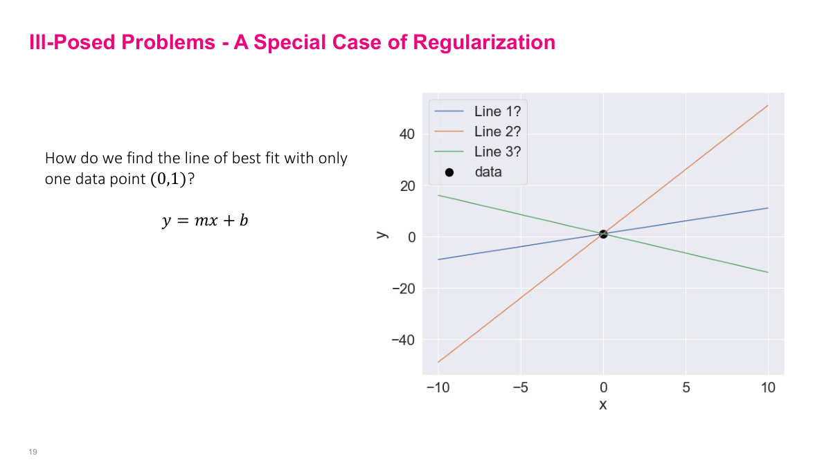
The first few things I'll go through are important to understand conceptually, although practically we may not use them as often. But they'll help you get intuition. The first problem regularization can deal with is the ill-posed problem. For example: how do we find the line of best fit with only one data point? You need more data points, and actually we can see that in the math. We can use the mean squared loss function we've been working with.

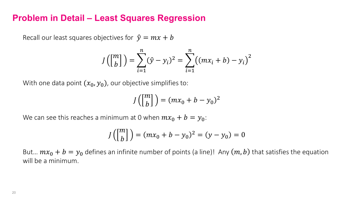
With a single data point (x₀, y₀), we plug it into our loss function. Since we only have one data point, no summation is needed. Because it's a squared function, the minimum occurs when the inside equals zero — basic quadratic function behavior. Setting the inside to zero gives us mx₀ + b = y₀, where x₀ and y₀ are constants. But we have two variables (m and b) in a linear combination that defines the line. A line has infinite points, so any point along that line satisfies this equation. As a result, any point along this line satisfies the minimum, but this doesn't help us because we want to find specific M and B parameters that fit the data well. This happens because we have more parameters than data points — two parameters but only one data point, giving us one equation for two unknowns. This doesn't happen often in deep learning because we usually have lots of data, and iterative algorithms like SGD handle this better than matrix inversion methods.

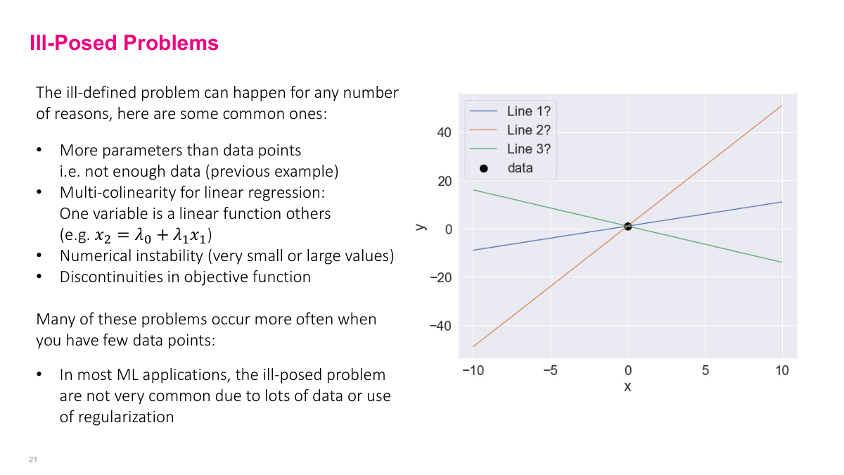
Related issues include having one variable being a function of other variables, numerical instability if numbers are very large or small, or discontinuity of the objective function. These are all things that happen when the optimization problem isn't formulated well mathematically, so you don't have a unique global minimum. As I mentioned, this isn't that common in deep learning because we usually have lots of data points, and stochastic gradient descent doesn't run into as many numerical stability issues as matrix inversion methods.

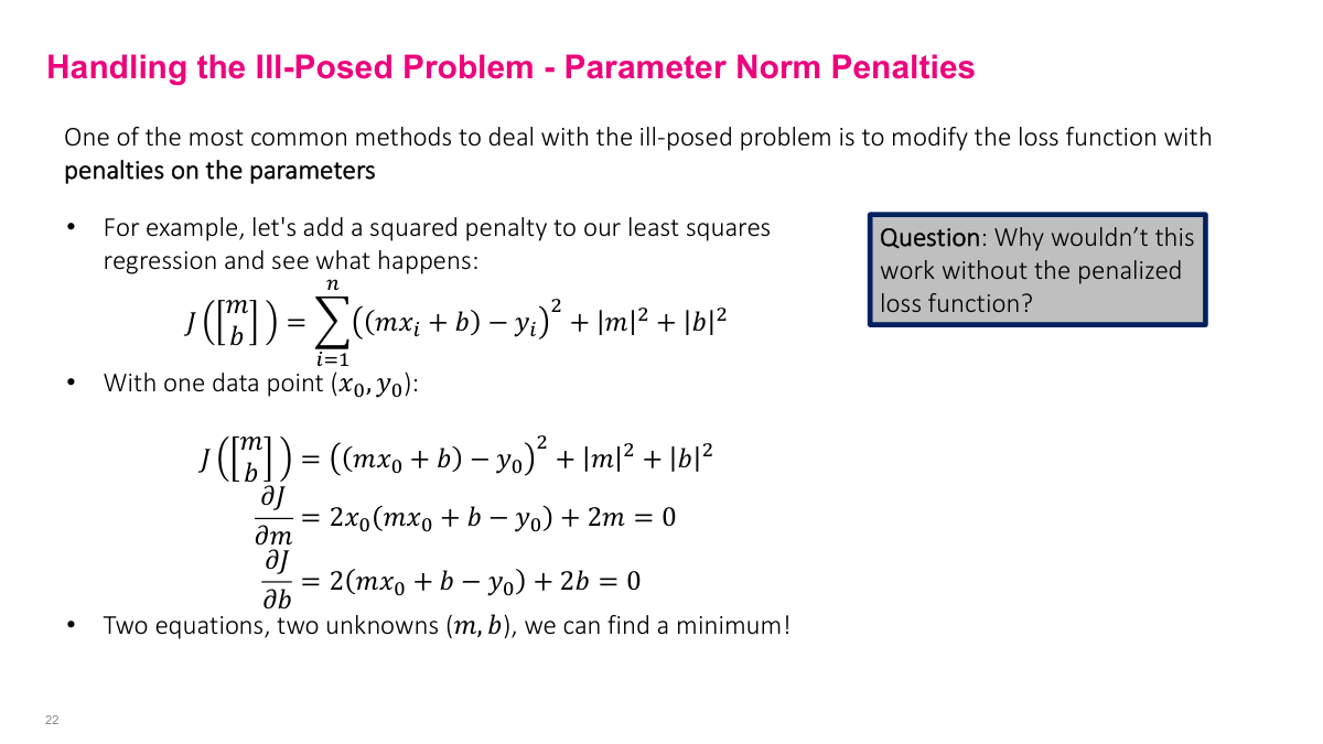
The way we generally handle this in ordinary least squares regression or linear regression (and you can do this in neural networks too) is through parameter norm penalties. In the objective function, we add additional terms that penalize the parameter values to ensure we get a unique solution. You can see the math here with x₀ and y₀. Before, we just had the main term, but now we're adding the m² and b² terms. When we take partial derivatives with respect to m and b, we get extra +2m and +2b terms. Now we have two equations and two unknowns, so we can find a minimum. Intuitively, adding these additional terms gives us the ability to find a minimum. Without these penalty terms, you won't have enough constraints to find the optimal solution — the equations become essentially the same equation, so you can't solve for a unique solution.

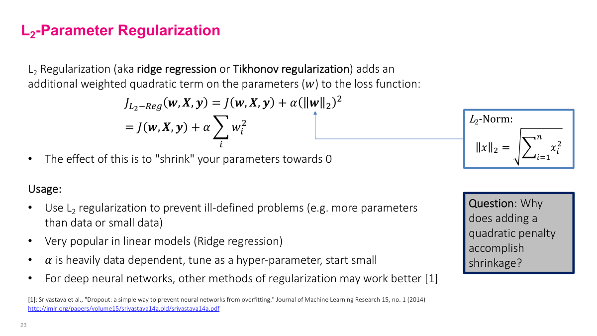
This is called L2 parameter regularization. In linear regression, it's also called ridge regression or Tikhonov regularization. If you use Scikit-learn, they have a ridge regression model that does exactly this for linear models. The idea is that we have our original objective function J, and we add penalty norms on all the parameters — basically the square of each parameter times some hyperparameter alpha. Alpha tunes how much regularization we want. Intuitively, this regularization shrinks all parameters towards zero. This helps prevent ill-posed problems, though that's not as relevant in deep learning. It's very popular in linear models. Alpha is heavily data-dependent — it's a hyperparameter you need to tune. When trying to minimize the generalization gap, alpha might make training error slightly worse but will reduce generalization error, so you want to find the sweet spot. We don't use it that much in deep neural networks, but the general concept of adding penalty terms to the objective function is an important part of regularization.

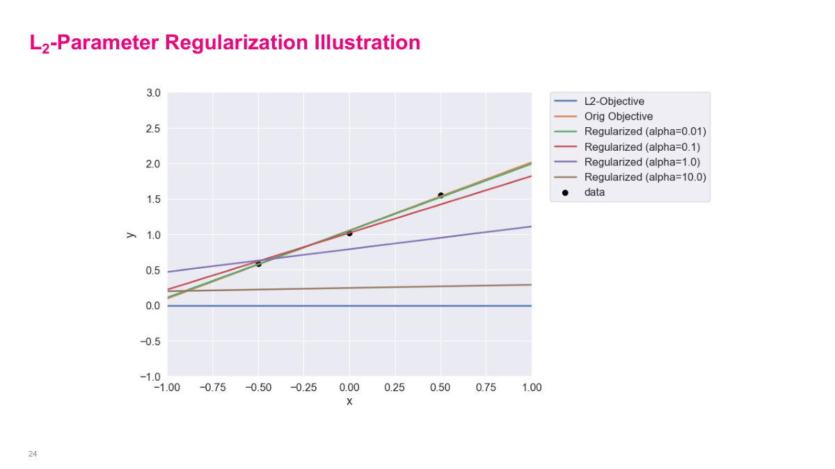
The orange line is the original objective — one of the best fit lines between these three data points. The blue line is what you'd get if you ignored the original objective and just had the penalty part — that would pick zero for each weight, so the line would be m=0, b=0. When you change alpha, it tries to find the balance between the original objective and the regularization objective. You can see the slope and intercept adjusting between the original line (orange) and the zero line (blue) depending on alpha. This gives you intuition about what alpha does — it interpolates or balances between the original objective and the regularization objective. As alpha becomes bigger, the regularization term takes priority and the result gets closer to the blue line. At alpha=10, it's much closer to the blue line and doesn't fit the original data very well.

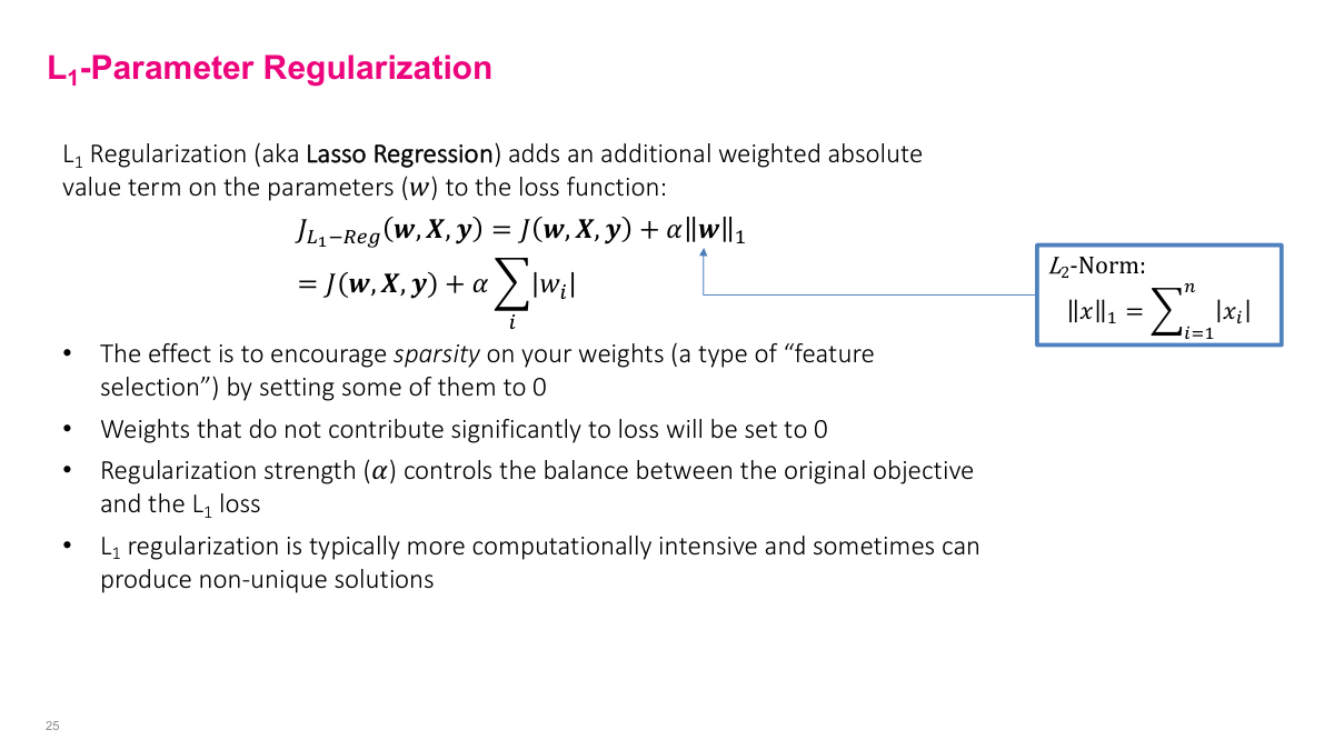
This is similar to L2 but uses L1 regularization, often called lasso regression. It's structurally similar except instead of having a square, it uses the L1 norm — the absolute value instead of the square. What this does is not just shrink parameters, but actually set them near to zero or very close to zero. Weights that don't contribute much will be more likely to be very close to zero. This acts as some kind of feature selection. Again, alpha controls how much you want to balance between the original objective and this regularization term. The last point about computational complexity is sometimes true, though not as important in deep learning when using stochastic gradient descent. Sometimes L1 regularization is more complex to compute when doing matrix inversions, but in SGD it's not that big of a deal.

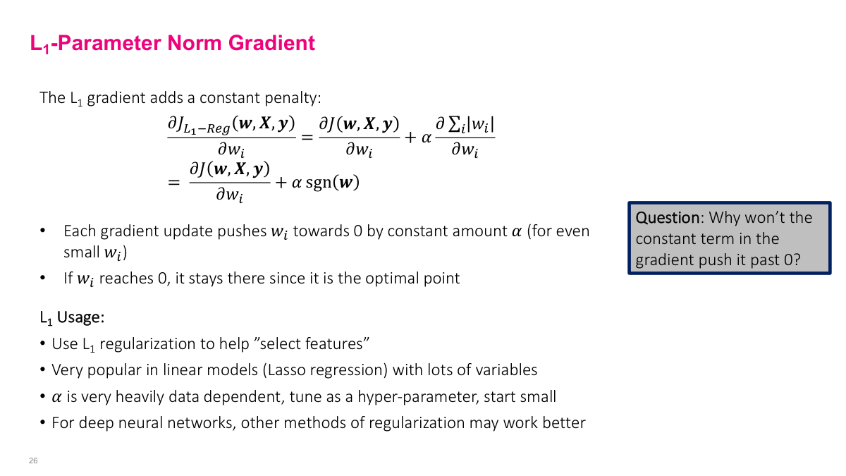
When we do the same exercise for L1, we get the original objective plus the sign of w. The sign is +1 or -1 depending on whether w is positive or negative — the derivative of absolute value is either -1 or +1. The idea is that the gradient will push the parameter towards zero by a constant amount every iteration. If it's positive, it'll subtract one every iteration; if it's negative, it'll add one. Once it reaches zero, it stays there. Why won't the constant term push it past zero to negative infinity? Because the sign flips. If it's positive, it keeps decreasing by one, but once it gets negative, it adds one instead. So it keeps pushing towards zero. L1 tends to look more like feature selection — it's not exactly feature selection, but it tends to do that. For neural networks with weight penalties on all weights, it's more complicated. You might get some zeros and some that are closer to zero, but what matters is whether it's helping solve your problem based on your validation set. For deep neural networks, we often don't use this much anymore, but the concept of adding extra terms to your objective function is important.

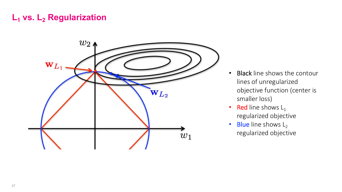
This diagram shows the optimization space in W1, W2. The black contour lines show the original objective function J — closer lines mean steeper slopes. The center is the absolute minimum. If you just had SGD, it would go to the center. But because you have L1 or L2 objective penalties, it also tries to pull towards these constraint regions. It finds the minimum on one of these curves that intersects with the objective. For L2, it tries to shrink both parameters to find the optimum, whereas the shape of the L1 regularization means you'll find a minimum that zeros out some values while L2 won't zero them out. It's the shape of the regularization term that causes this difference. This visualization helps explain why L1 zeros out values while L2 just shrinks them.

Another common regularization technique, especially for different types of data, is data augmentation. Data is the foundation of what the model learns, so adding more data is good. We can add synthetic data — even though we don't have totally new data points, if we can add synthetic data somehow, it could improve model performance. The idea is to augment your training set with new synthetic data points while leaving validation and test sets alone. Add more data to your training set, then make sure it still works on your validation test set. If it doesn't improve things, don't do it. It's not universally good to add synthetic data because it depends on whether the synthetic data actually matches the real data distribution. You could add synthetic data that's totally different and cause your model to go haywire. Sometimes it's easier to find extra real data instead of synthetic data, but synthetic data is very useful in certain domains.

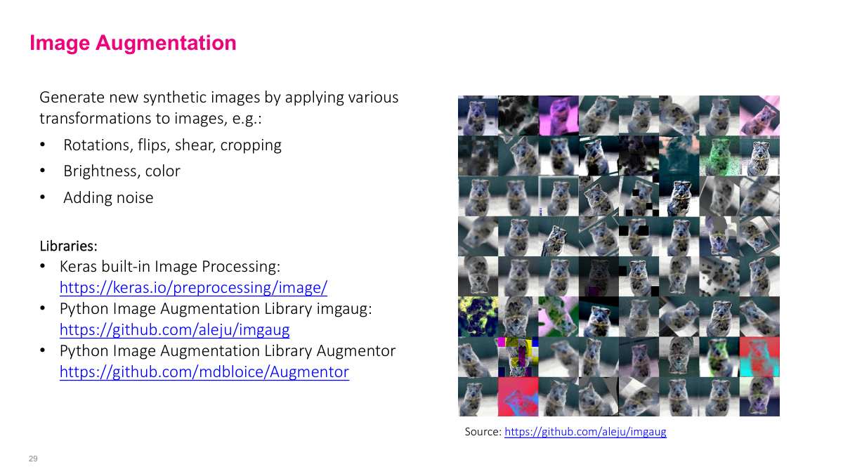
Synthetic data is very useful for images. There are many libraries available, and you can see some data augmentations in the picture. Images are particularly good for augmentation because you can do simple transformations that are still valid images. Rotate it slightly, flip it, change the color or lighting — those are still valid pictures. If you took photos under certain lighting conditions, adding these variations will actually increase generalization and help the model learn something broader, not be so overfit to your specific training dataset. Generally it works really well. You usually have some domain knowledge about what a good data point looks like, so you can add good augmentation. Modern approaches use like a dozen different transformations randomly throughout the dataset to augment data.

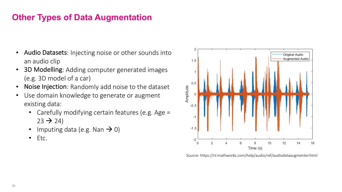
You can do similar things for other data types. For audio datasets, you can add noise — hopefully you should still be able to pick up voices. If you've only heard voices in a quiet classroom, it's different from hearing on a noisy street, so adding noise makes sense. For 3D modeling, you can use 3D models to generate more data points. You can add certain types of noise to datasets too. But be careful with tabular data — changing age from 23 to 24 might be okay, but changing from 17 to 18 or 17 to 19 might cross important thresholds your model should learn. Don't randomly add data points that don't follow the data distribution you have. Adding noise helps prevent overfitting — it's not learning the specific noise, just the general signal.

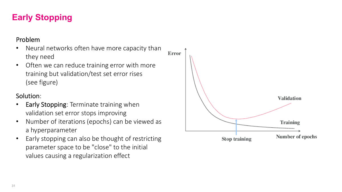
Another type of regularization is early stopping. If you train for many epochs, we've seen training curves where at some point your validation error starts going up even though training error goes down. One thing you can do is just stop training at the optimal point. This is very easy to do. Most modern models support checkpointing — after every epoch or every few epochs, it saves the model weights. Even if you set it for 100 epochs and trained overnight, you have all the checkpoints in between. You can look at the graph and pick the model from the optimal point. You can think of this as regularization because stopping early constrains how far you can move from your initial solution — you can't go too far because you don't have enough epochs. Is it possible to reach a local minimum instead of global minimum? Everything we do finds local minimums — we almost never find global minimums with million-parameter models. One intuition for why bigger models work better is that the bigger the model, the more likely you'll find a local minimum that's pretty good. With too few parameters, you need to find exactly the right minimum. With over-parameterized models, most local minimums are actually pretty good.

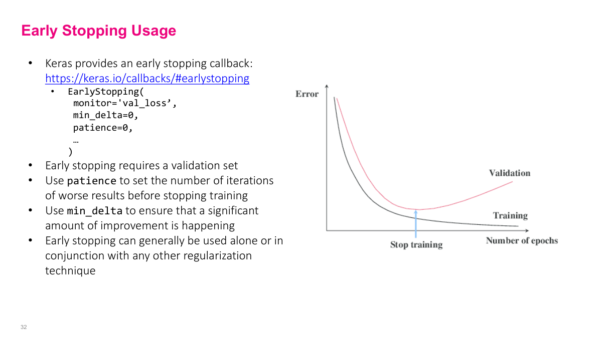
In Keras, there's actually a callback you can add to do early stopping, and most modern frameworks have this feature. There's also a checkpointing feature you can use. You can look at the details of how to use it, but there are parameters for how long you wait before stopping and how big a difference you want to see before it decides not much has changed.

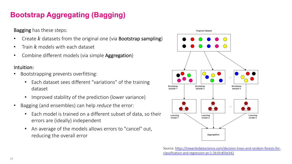
Bootstrap aggregating (bagging) is a combination of two things: bootstrap sampling (sampling with replacement to have subsets of the data) and training models on each subset, then aggregating them through some function. This is good because we ensemble things. We have ensembles with hopefully independent characteristics that aren't correlated because we're sampling random samples of the dataset. When ensembling using multiple models and combining them through aggregation, as long as they're independent, there's a tendency for errors to cancel out. This probably overfits on this dataset or is idiosyncratic for this dataset, but when you aggregate them together, especially if you have enough different samples, a lot of the errors will cancel out. So when you aggregate, you'll have overall lower variance and often better bias as well.

Bootstrapping is randomly sampling with replacement, and aggregation is training the model for each subset of data then aggregating them. Classification can use votes, regression can use the average of all predictions. This is pretty much the same idea as random forest.

Random forest uses bagging. One interesting thing with bagging is that it doesn't matter how strong or high capacity your model is for each of the models in each data sample. Random forest uses a pretty weak model (weak learners) like a decision tree, and combines many decision trees to get a much better overall model. You can do the same with neural networks — train small neural networks on different samples and combine them. This is a perfectly valid technique and usually gives more stability because bootstrapping helps with variance of the output. Dropout is often used more. Ensembles in general are good in practice. Even without bagging specifically, if you really care about low variance output, you can train multiple models with different architectures, hyperparameters, or datasets and aggregate the output to minimize the effect of overfitting to one particular architecture, dataset, or training run. Why don't we use large deep nets with bagging? It's computationally expensive. Each net takes several hours to train, so doing 10 different nets needs 10 times the resources or time. With modern models like Grok 3 using tens of thousands of GPUs for months, you can't train five different versions.

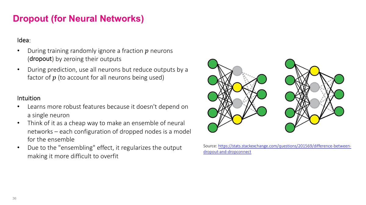
Dropout is probably what you'll use most. It's the most popular regularization technique. Dropout is actually a simple idea: during training, for any layer you put dropout on, it randomly zeros out or ignores a random proportion p of nodes in the forward pass and correspondingly in the backward pass. In this example, I put dropout on the middle layer with p=0.5 (50%). So randomly, during forward pass, I'm going to drop two of these nodes and only use the other two. This seems weird — why randomly turn off stuff? One iteration, I randomly turn off these nodes and don't propagate any weights forward or do backward updates through these, just use these two nodes. Next forward pass, I'll select a different 50%, say these two yellow ones. Some intuition: it makes sure when neural networks are learning, they're not so dependent on any single neuron. You can imagine the model being overly dependent on one specific neuron to get the right answer, which isn't robust — if a weird input oversaturates or zeros out that neuron, you might have problems. So you want to distribute learning across multiple neurons. If you randomly turn it off, it forces the neural network to change weights so other neurons can participate in the prediction. Another intuition is that it's a cheap way to ensemble — you don't want to train five models overnight, but this neural network and this neural network are different. It's like averaging between all the different variations.

You can have a regular dense layer, then add dropout, dense, dropout, dense, dropout — that's generally how it works. One key hyperparameter is p, and you may need to increase the number of epochs because you're only training a subset of the weights at a time. This is probably the most common thing you'll see. I'd recommend if you're thinking about regularization, start with dropout and put it on all or most of the layers in your neural network, then tune the p parameter. You can probably have the same p for most layers. Maybe start with something small like 10% if you're not seeing much overfitting, and increase to 50% or potentially more, depending on how much capacity your network has. During inference, you have to adjust the magnitude because during training it only sees half the inputs, but during test time it sees all inputs. The magnitude will be roughly twice as large, which could saturate the node. You need to adjust by some function of how many things you drop — I think it's one over p.

Actually, the best kind of regularization is adding more data. You can imagine we're building a cat classifier to distinguish cat versus dog. Which scenario is most likely to overfit: 1,000 images, 10,000 images, a million images, or a billion images? The more data you have, the less likely you are to overfit. So someone like Instagram, who has billions of images, maybe doesn't need to think about regularization as much, at least when doing really large training runs (though I'm sure they have some regularization). The best case is having every single possible data that you could ever see, so the train distribution exactly matches your prediction distribution. But in any case, the more data we have, the more likely that what we see in the wild will match something in our training set, and the better our model will perform.

Let me quickly go through the review questions. What is regularization? It's a set of strategies to avoid overfitting — any modifications to the machine learning algorithm to minimize the gap between train and test. What are norm penalties? L1 and L2 norm penalties that add extra terms to the loss function to penalize certain aspects. What is data augmentation? Adding synthetic data from the original dataset, other than generating completely new data. It's adding synthetic data to your training dataset hoping the model learns more generalization. It's very dependent on how you define the synthetic data. What is bagging? Bootstrap samples with replacement, train different models on different samples, then aggregate them together through majority vote or averaging. What is dropout? During training, we randomly ignore a fraction p of neurons by zeroing out their outputs. The key thing is that because we're zeroing some out, during test time we have to adjust by some function of how many things we drop, because the magnitude into the destination changes significantly. What is the ideal type of regularization? Practically dropout is what you'll use, but the ideal type is adding more data points. If you have every single data point theoretically, then you technically can't overfit because you've seen everything.

This slide summarizes the key regularization techniques we've covered: L1 and L2 parameter penalties, data augmentation, early stopping, bagging, and dropout. Each serves to reduce the generalization gap in different ways.

This references slide lists the academic sources and foundational papers for the regularization techniques discussed in this lecture.