Lecture 06: NLP and Representation Learning

This lecture covers representation learning and text representations. We look at some key ideas: what representation learning is, the manifold hypothesis, vector space models, cosine similarity, word embeddings, and t-SNE for visualization. Many of the specific techniques here are somewhat outdated with the advent of large language models, but the underlying concepts remain foundational.

The key questions for this section: What is representation learning? What is the manifold hypothesis? What is a vector space model? What is cosine similarity? What is the curse of dimensionality? What is a word embedding? How do we model a document using word embeddings? What is t-SNE and what is it used for?

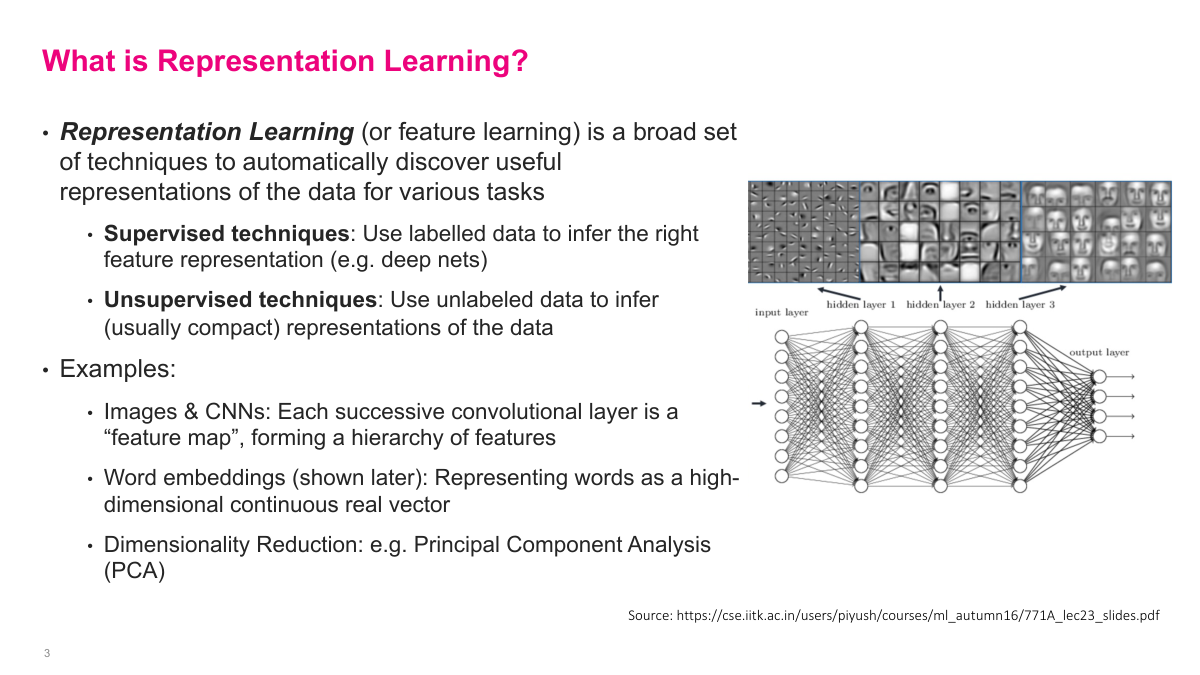
Representation learning, or feature learning, is a broad set of techniques for automatically discovering useful representations of data. Supervised techniques like transfer learning use labeled data to learn feature representations -- each successive layer of a CNN produces a feature map, forming a hierarchy of learned features without us explicitly specifying them. Unsupervised techniques learn compact representations from unlabeled data. A 1000x1000x3 image with three million dimensions can be compressed down to several hundred dimensions while retaining most of the useful information. Word embeddings represent words as compact continuous vectors, and even today's large language models use the same concept to represent text in a 500-dimensional vector. PCA is another, simpler form of representation learning using linear transformations. The core idea is always the same: take the data distribution and represent it in a much more compact way.

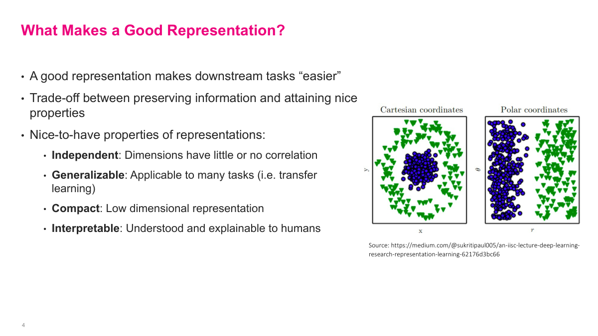
There is no single mathematical criterion for a good representation -- generally, it should make downstream tasks easier. There are trade-offs between how much information it retains and the properties it has. Some nice-to-have properties: independent dimensions with little correlation, which is especially useful for linear classifiers; generalizable to many tasks (transfer learning); compact, reducing millions of dimensions to perhaps a few hundred; and interpretable, though that is more of a bonus than a requirement. The diagram on the right illustrates this nicely -- in Cartesian coordinates, two classes overlap, but switching to polar coordinates makes them cleanly separable. A good representation is one that makes the problem you are solving easier.

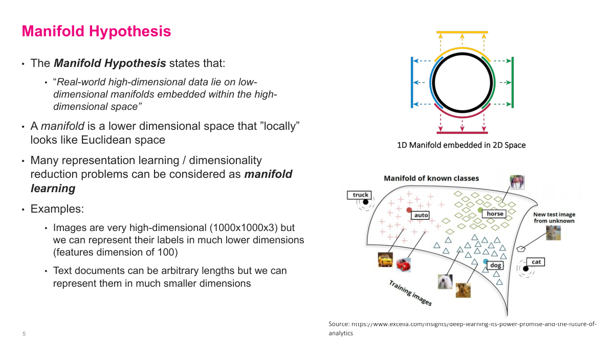
The manifold hypothesis is a key idea in deep learning: real-world high-dimensional data lies on low-dimensional manifolds embedded within the high-dimensional space. A 1000x1000x3 image has three million dimensions, but the vast majority of possible values in that space are just random noise. The actual images we care about can be represented on a much smaller surface. Think of a sphere in 3D space -- the surface itself is a 2D manifold that can be mapped to two dimensions. Similarly, those three-million-dimensional images can often be reduced to around 100 dimensions while retaining their essential properties. This is arguably the thesis of why deep learning works: the last layer of a classifier might only have a few hundred dimensions, yet it still classifies accurately because the network learned to project onto the relevant manifold. Text documents work the same way -- arbitrary-length text can be compressed into a relatively small vector. Representation learning and dimensionality reduction can both be viewed as forms of manifold learning.

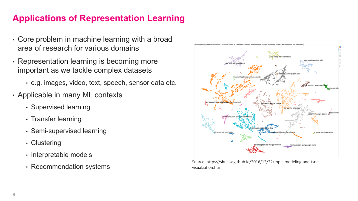
Representation learning is a core problem in machine learning with applications across many domains -- images, video, text, speech, sensor data. It shows up in supervised learning, transfer learning, semi-supervised learning, clustering, interpretable models, and recommendation systems. As we tackle increasingly high-dimensional and complex datasets, learning good representations becomes ever more important.

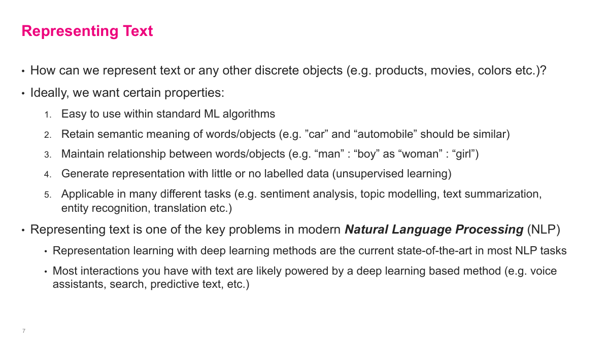
Representing text has been one of the hardest problems in machine learning. Words are discrete objects -- you cannot simply map them onto the real number line. We want representations that are easy to use in ML algorithms, retain semantic meaning (so "car" and "automobile" are similar), maintain relationships between words (like "man" to "boy" as "woman" to "girl"), can be generated with little or no labeled data, and are applicable across many tasks -- sentiment analysis, topic modeling, text summarization, and more. Large language models have largely solved this problem, but the underlying concepts of how we got there are still worth understanding. Deep learning methods made huge leaps in the 2010s, and today pretty much anything involving text is powered by deep learning.

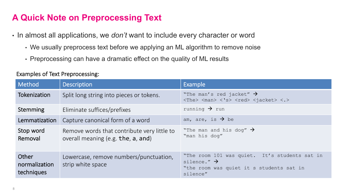
Even in the age of large language models, text preprocessing matters. The most important technique that remains relevant today is tokenization -- splitting text into discrete tokens that the model processes. Large language models predict one token at a time, and tokens are roughly words but not exactly. Earlier NLP relied on additional preprocessing to simplify the problem: stemming (dropping conjugations, so "running" becomes "run"), lemmatization (mapping to canonical forms, so "am", "are", "is" all become "be"), stop word removal (dropping words like "the" and "and" that contribute little meaning), and other normalization like lowercasing and removing punctuation. Nowadays we pump everything into large language models and they handle it, but tokenization remains a critical hyperparameter even for modern systems.

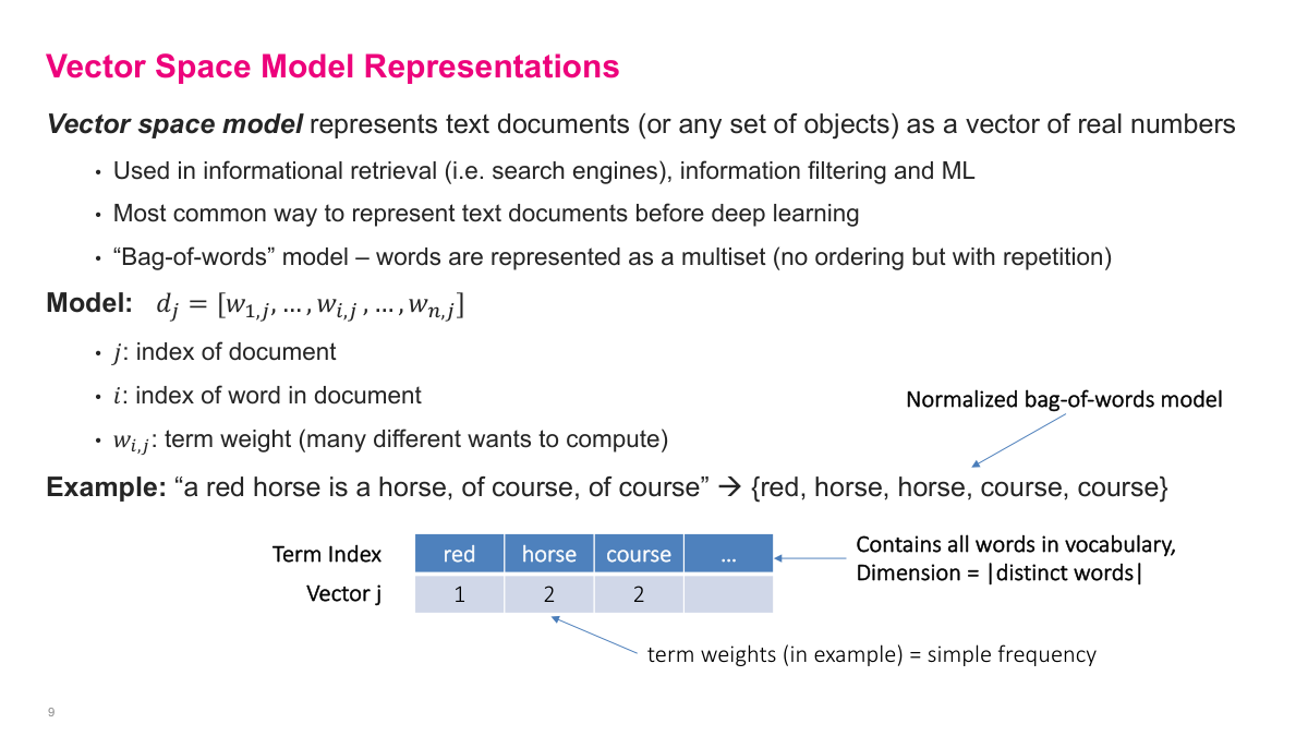
The vector space model was the most common way to represent text before deep learning. The idea is simple: represent a document as a multiset of words -- count how many times each word appears, ignoring order. For example, "the red horse is a horse, of course, of course" becomes the counts: red=1, horse=2, course=2. The resulting vector has one dimension per word in your vocabulary. With a typical English vocabulary of 10,000-15,000 words, this vector is very long and very sparse -- only a handful of entries are non-zero for any given document. This sparsity is actually useful for storage since you only need to represent the non-zero entries, but it creates challenges for comparison and downstream ML tasks. The vector space model can also represent any discrete objects, not just text -- products, colors, categorical variables.

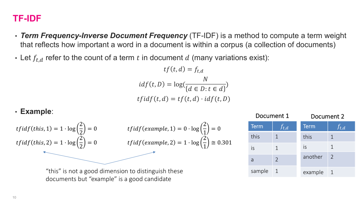
TF-IDF (Term Frequency-Inverse Document Frequency) modifies the raw word counts so the weighting reflects how informative a term actually is. Term frequency is just the count of a word in a document. Inverse document frequency down-weights terms that appear across many documents -- if a word like "this" appears in every document, it gets a TF-IDF of zero because log(N/N) = 0. A word like "example" that appears in only one of two documents gets a non-zero IDF, so it receives a higher weight. The intuition: rare terms are more informative for distinguishing documents, while common terms that appear everywhere carry little signal. You multiply TF by IDF to get the final weight. This is essentially feature extraction -- figuring out which terms matter for differentiating documents. Not used much anymore with deep learning and massive computation available, but it is an interesting concept from the pre-deep-learning era.

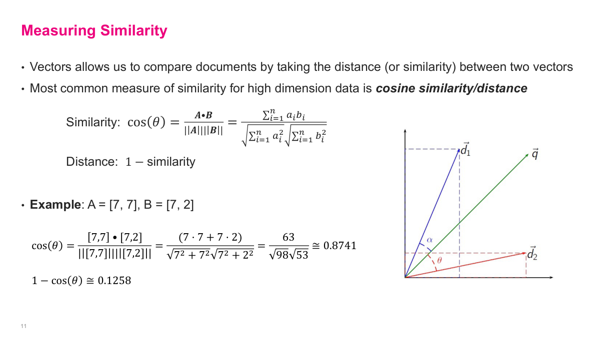
Once you have vector representations -- whether several hundred or 10,000 dimensions -- you need a way to compare them. The most common measure for high-dimensional data is cosine similarity, which measures the cosine of the angle between two vectors. It is straightforward to compute and works well even for very high-dimensional vectors. The standard Euclidean distance that we learn in school does not work well in high dimensions due to the curse of dimensionality, which we cover next. Cosine distance is simply 1 minus the cosine similarity.

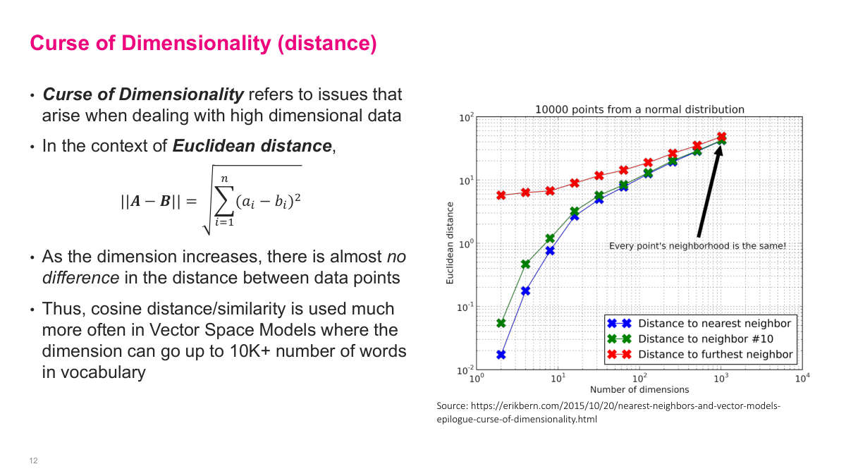
The curse of dimensionality has multiple forms. In terms of distance: as you increase the number of dimensions, the average Euclidean distance between the nearest neighbor and the furthest neighbor converges to nearly the same value. You can see this in the chart -- as dimensions increase, the distance to the nearest neighbor and furthest neighbor approach each other. If you cannot distinguish things that are far apart from things that are close together, the distance metric is useless. This is why cosine similarity is preferred over Euclidean distance in vector space models with 10,000+ dimensions, especially with sparse vectors.

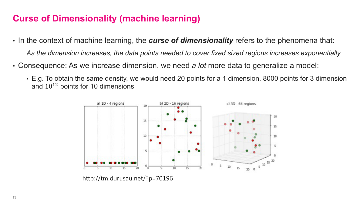
The other form of the curse of dimensionality relates to data coverage. As dimensions increase, the number of data points needed to densely cover the space increases exponentially. With 20 data points in one dimension, you cover the space well. In two dimensions with the same 20 points, there are large gaps. In three dimensions it gets worse. To maintain the same density, you need 20 points for 1 dimension, 8,000 for 3 dimensions, and 10^12 (a trillion) for just 10 dimensions -- which is completely infeasible. Anything exponential is simply not physically realizable, which is why working directly in very high-dimensional spaces is problematic.

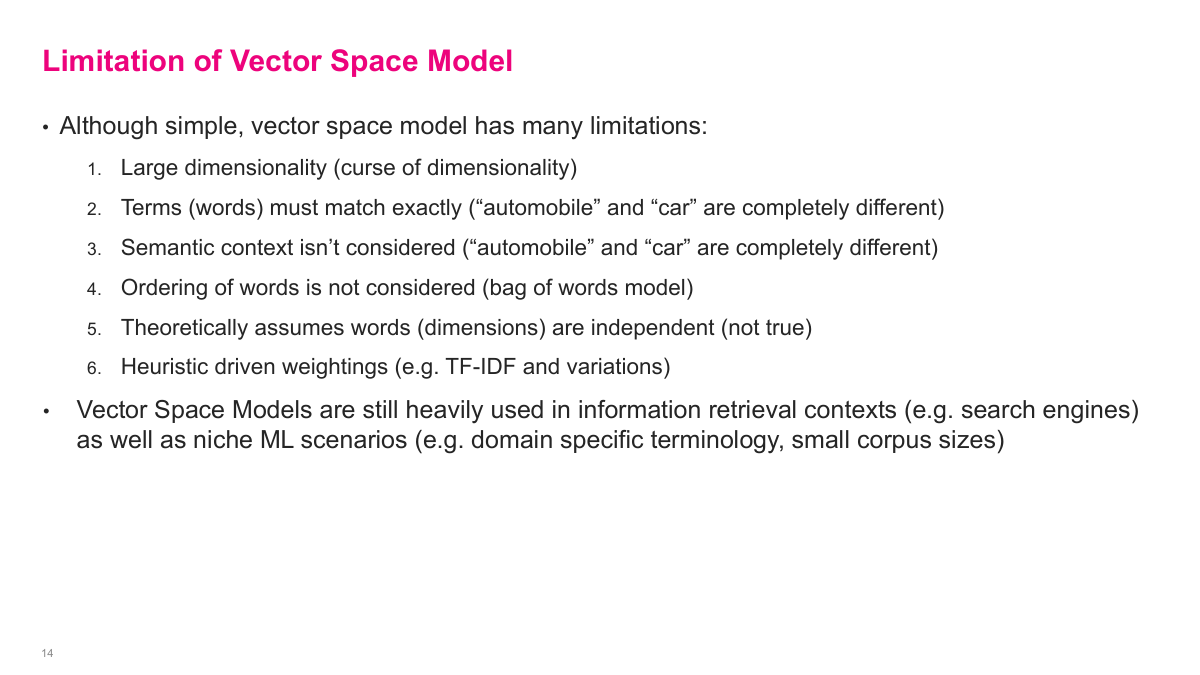
The vector space model has several key limitations. First, large dimensionality and the curse of dimensionality -- 10,000+ dimensional vectors just are not practical. Second, terms must match exactly: "car" and "automobile" are completely different entries in the vector, so you miss that synonymy. Third, semantic context is not considered. Fourth, word ordering is ignored since it is a bag-of-words model. Fifth, it assumes words are independent, which is not true. Sixth, the weightings like TF-IDF are heuristic-driven rather than learned. The trend in modern machine learning is to move away from manual feature engineering and learn representations instead. Vector space models are still used in some search and information retrieval contexts, but rarely in ML scenarios now. The concepts that remain important are cosine similarity and understanding why these simpler approaches fall short.

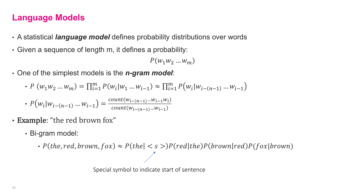
A statistical language model defines probability distributions over sequences of words -- the goal is to predict what the next word or token will be. One of the simplest approaches is the n-gram model. For a sequence of words w1 to wm, we approximate the joint probability as a product of conditional probabilities, where each word is conditioned on the previous n-1 words. In the bi-gram case, we predict each word based only on the previous word. For example, P("the red brown fox") is approximated as P("the"|start) P("red"|"the") P("brown"|"red") * P("fox"|"brown"). A simple way to estimate these probabilities is by counting: how many times have I seen "fox" followed by "jump" divided by how many times I've seen "fox" total? Google used this n-gram counting approach for early Google Translate and it worked surprisingly well. But as you increase the context window, the number of possible sequences grows exponentially, making pure counting infeasible. Large language models solve this by using deep neural networks with much larger context windows -- thousands of tokens -- to produce probability distributions over what comes next.

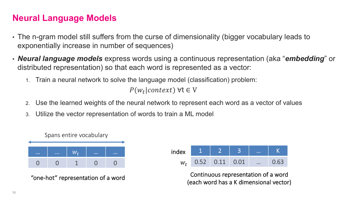
N-gram models suffer from the curse of dimensionality -- increasing the context window causes an exponential blowup in possible sequences. Neural language models address this by expressing words as continuous representations, or embeddings, instead of sparse one-hot vectors. We train a neural network to solve the language model classification problem: given some context, predict the probability distribution over the next word using a softmax output layer. The key insight is that the internal weights of this neural network become our representation of the text. Going from a one-hot encoded vector with mostly zeros to a dense, continuous, K-dimensional embedding where every dimension carries information -- that is the fundamental shift. Where a word sits in this K-dimensional space encodes a lot about what that word means.

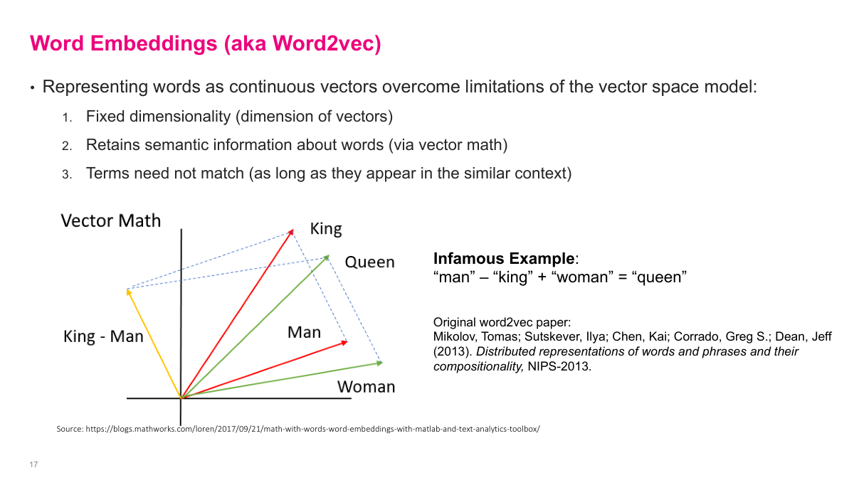
Word embeddings, popularized around 2011, were a major breakthrough for working with text. They compress any word into a fixed-dimension vector -- say 50 or 100 dimensions -- while retaining semantic meaning. Words like "car" and "automobile" end up close together in the embedding space. The famous example: take the vector for "man", subtract "king", add "woman", and you get something very close to "queen". The distances between vectors in the space carry semantic meaning. This was a big deal because it meant you could train word embeddings on a large body of text, then use those pre-trained embeddings for any downstream task. Instead of dealing with the custom preprocessing of vector space models, you just plug in fixed-dimensional vectors and feed them to whatever classifier you want. Word embeddings are one of the direct precursors to large language models.

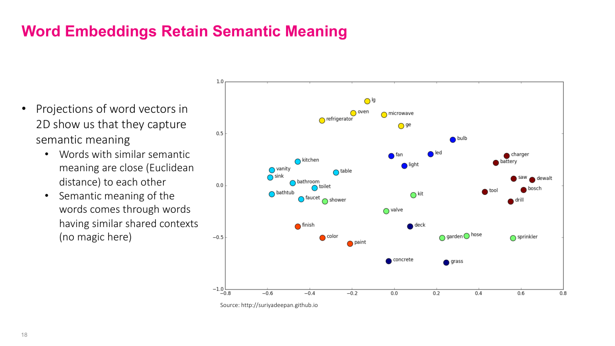
This 2D visualization of word embeddings shows that semantically similar words cluster together in the vector space. Words like "bathroom", "sink", "kitchen", and "bathtub" are grouped together, while "battery", "charger", "saw", "drill", and "Bosch" form a separate cluster of tools and power equipment. The semantic meaning emerges naturally from words sharing similar contexts in the training data -- there is no magic. This property of retaining semantic relationships was a major breakthrough in machine learning because it allowed us to work with text much more effectively.

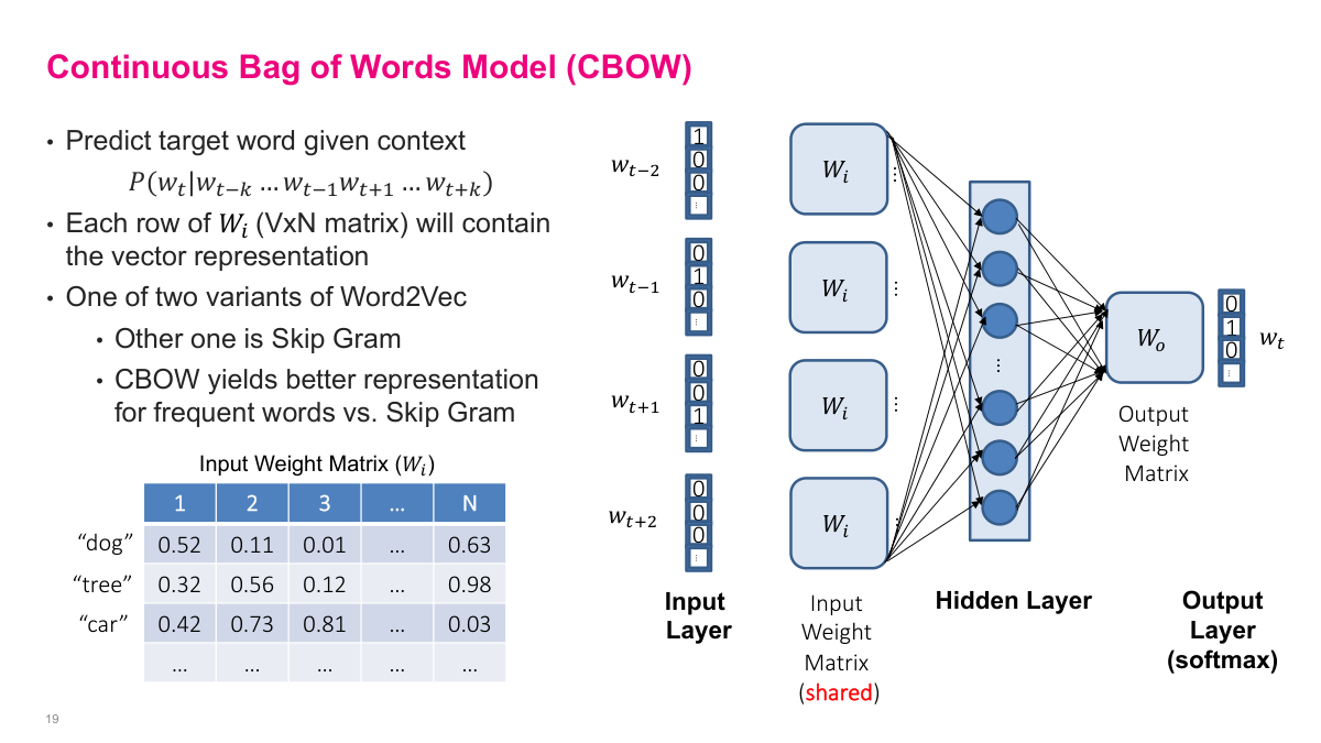
The Continuous Bag of Words (CBOW) model is one of two Word2Vec variants (the other being Skip-Gram). Instead of predicting the next word from previous words, CBOW predicts a target word from its surrounding context words. The input is the words around the target -- for example, w(t-2), w(t-1), w(t+1), w(t+2) -- and the output is a softmax over the entire vocabulary predicting the target word. The architecture is a single hidden layer feed-forward neural network with a shared input weight matrix. Each row of this VxN weight matrix becomes the vector representation for the corresponding word. The "shared" part is key: whether a word appears in the first context position or the third, it uses the same weights. CBOW tends to yield better representations for frequent words compared to Skip-Gram.

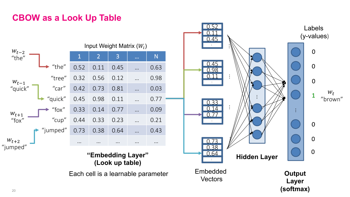
The first layer of CBOW is essentially a lookup table, often called an embedding layer. For each context word, you look up its row in the weight matrix to get an N-dimensional vector. These vectors feed into the hidden layer, which connects to a softmax output predicting the target word. In the example, the context words "the", "quick", "fox", "jumped" each look up their corresponding row, producing four embedded vectors that are fed into the network to predict "brown". The entire weight matrix is shared across all context positions and consists of learnable parameters -- initialized randomly and updated via backpropagation. As you train over a large body of text, this lookup table learns meaningful representations for each word, placing semantically related words near each other in the embedding space.

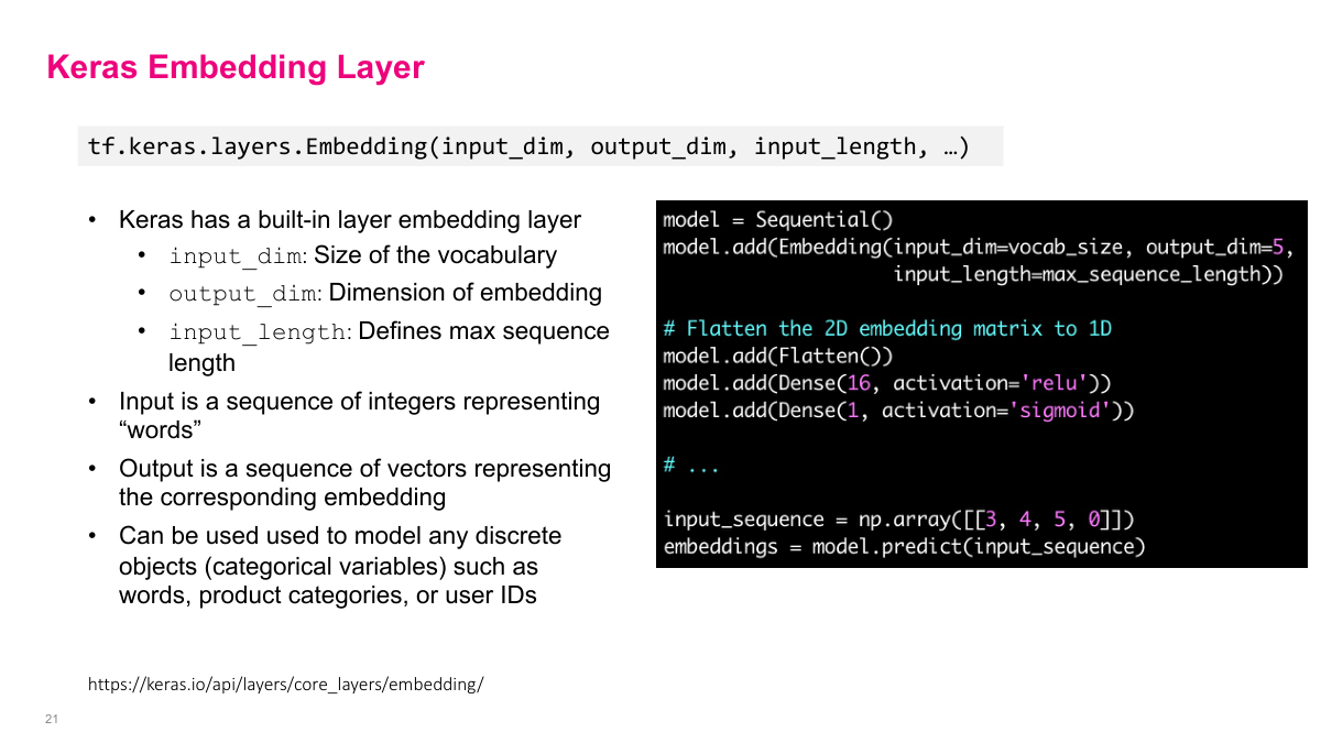
Keras provides a built-in Embedding layer that implements the same lookup table concept. You specify input_dim (vocabulary size -- the height of the table), output_dim (embedding dimension -- the width), and input_length (max sequence length). The input is a sequence of integers representing words, and the output is the corresponding sequence of embedding vectors. This layer is not limited to words -- you can embed any discrete objects like product IDs, categories, or user IDs. In the context of large language models, the same idea applies: internal weights of the network represent a span of text as a dense vector. OpenAI models, for instance, produce 768-dimensional embeddings that you can feed into a simple classifier for tasks like sentiment analysis, or compare for text similarity in applications like retrieval-augmented generation.

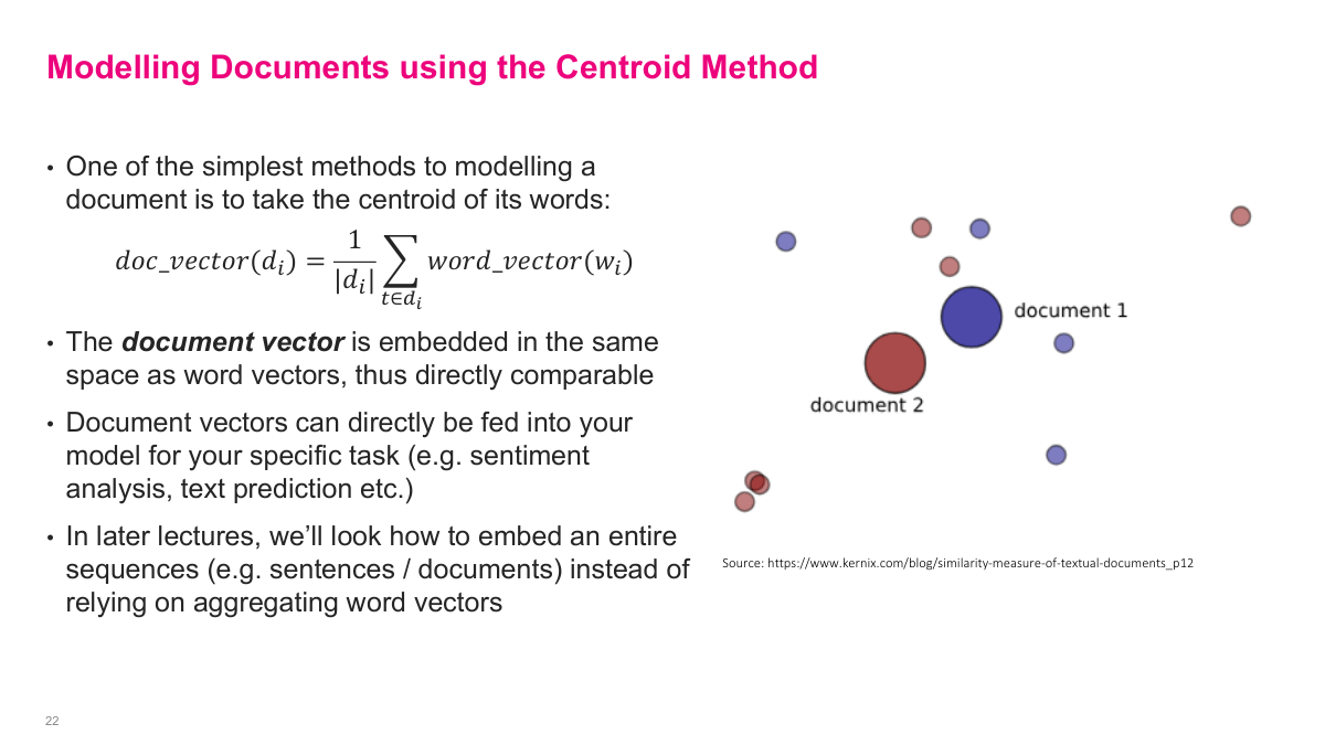
Word embeddings give you a vector per word, but often you need to represent an entire document or sentence. One of the simplest approaches is the centroid method: take the average of all the word vectors in the document. The resulting document vector lives in the same embedding space as the word vectors, so you can directly compare documents or feed them into a classifier. It is a basic approach, and later lectures cover more sophisticated methods for embedding entire sequences, but averaging works surprisingly well as a starting point.

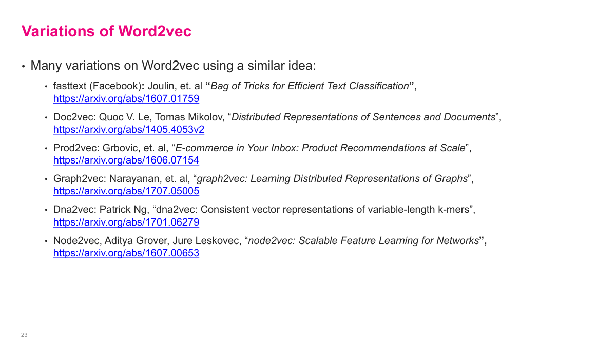
The Word2Vec idea of learning dense, continuous vector representations for discrete objects has spawned many variations. fastText from Facebook is an improved word embedding method. Doc2Vec extends the concept to entire documents. Prod2Vec applies it to e-commerce products. Graph2Vec and Node2Vec learn representations for graph structures. Even DNA sequences have been embedded with dna2vec. The core idea is always the same: take discrete objects, learn a fixed-dimension dense vector for each, and use those vectors for downstream tasks. This is a fundamental concept in machine learning and representation learning.

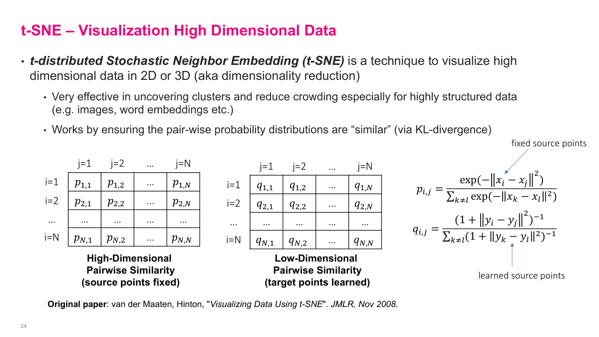
t-SNE (t-distributed Stochastic Neighbor Embedding) is a technique for visualizing high-dimensional data in 2D or 3D. Even 10 dimensions are hard to visualize, and we often work with hundreds. The algorithm works by computing pairwise similarities between all data points in the original high-dimensional space, creating a similarity matrix. It then creates a corresponding low-dimensional representation (the y vectors) with its own pairwise similarity matrix. The low-dimensional points are learnable parameters -- you use stochastic gradient descent with KL divergence as the loss function to make the two similarity matrices match as closely as possible. If the low-dimensional representation is good, the pairwise distances in 2D should mirror the pairwise distances in the original space. t-SNE is especially effective at uncovering clusters in highly structured data like images and word embeddings.

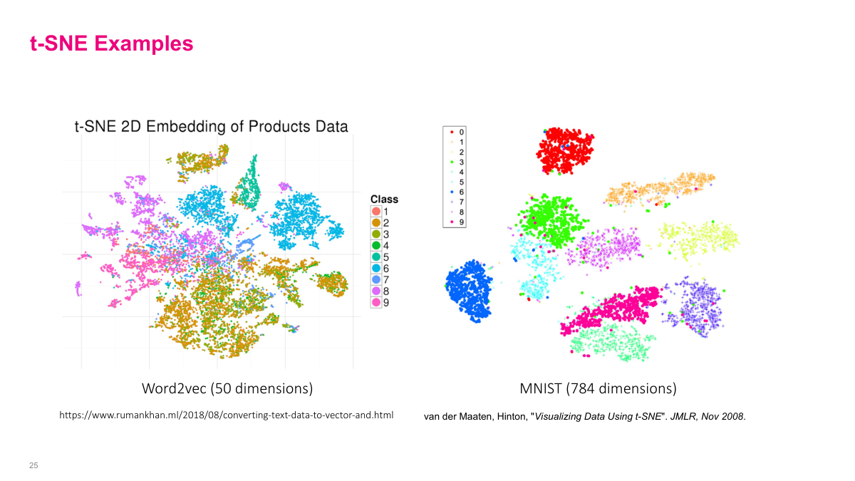
Two examples of t-SNE in action. On the left, 50-dimensional Word2Vec product embeddings are projected to 2D, and you can see products of similar classes clustering together based purely on the learned context. On the right, MNIST handwritten digit images (784 raw pixel dimensions) are projected to 2D, and the digit classes separate into distinct clusters. Some digits that look similar to each other, like 4 and 9, end up closer together. t-SNE is a powerful tool for visualizing and debugging high-dimensional representations.

There are many t-SNE implementations available: the original author's code in Matlab, Python, Java, and others; TensorBoard's embedding projector which supports t-SNE, PCA, and custom projections; scikit-learn; a JavaScript implementation by Karpathy; and a parallel multi-core version. A more modern alternative is UMAP, which gives similar results but is algorithmically more efficient. The main limitation of t-SNE is that it is O(n^2) -- it computes all pairwise distances, so with a million data points it becomes infeasible. For smaller datasets, t-SNE works well; for larger ones, consider UMAP.

Representation learning is a key area of machine learning focused on learning compact representations of high-dimensional data rather than hand-engineering features. The manifold hypothesis says high-dimensional data lies on lower-dimensional manifolds -- most of those dimensions are redundant. The vector space model represents text as sparse word-count vectors, but suffers from high dimensionality, no semantic understanding, and independence assumptions. Cosine similarity measures the angle between vectors and works much better than Euclidean distance in high dimensions due to the curse of dimensionality. Word embeddings are dense, continuous, fixed-dimension representations where semantic meaning is captured through shared context -- unlike one-hot vectors, every dimension carries information. To model an entire document with word embeddings, you can take the centroid (average) of the word vectors. t-SNE is a dimensionality reduction technique for visualizing high-dimensional data in 2D or 3D by matching pairwise similarity distributions between the high and low dimensional representations.