Lecture 07: Recurrent Neural Networks

In this section, I introduce recurrent neural networks as the standard way to model sequential data. The big ideas are straightforward: sequential problems have order, simple recurrent networks struggle with training instability, and LSTMs add gates and memory to make these models work much better in practice. My goal here is not to exhaust the topic, but to give you a durable mental model for how recurrent architectures process information over time.

These are the questions that organize the whole section. I want you to be able to distinguish the major types of sequential problems, define what an RNN is, explain why simple recurrent networks are hard to train, and describe what an LSTM adds. If you can answer those five questions cleanly at the end, then you have the conceptual foundation that matters.

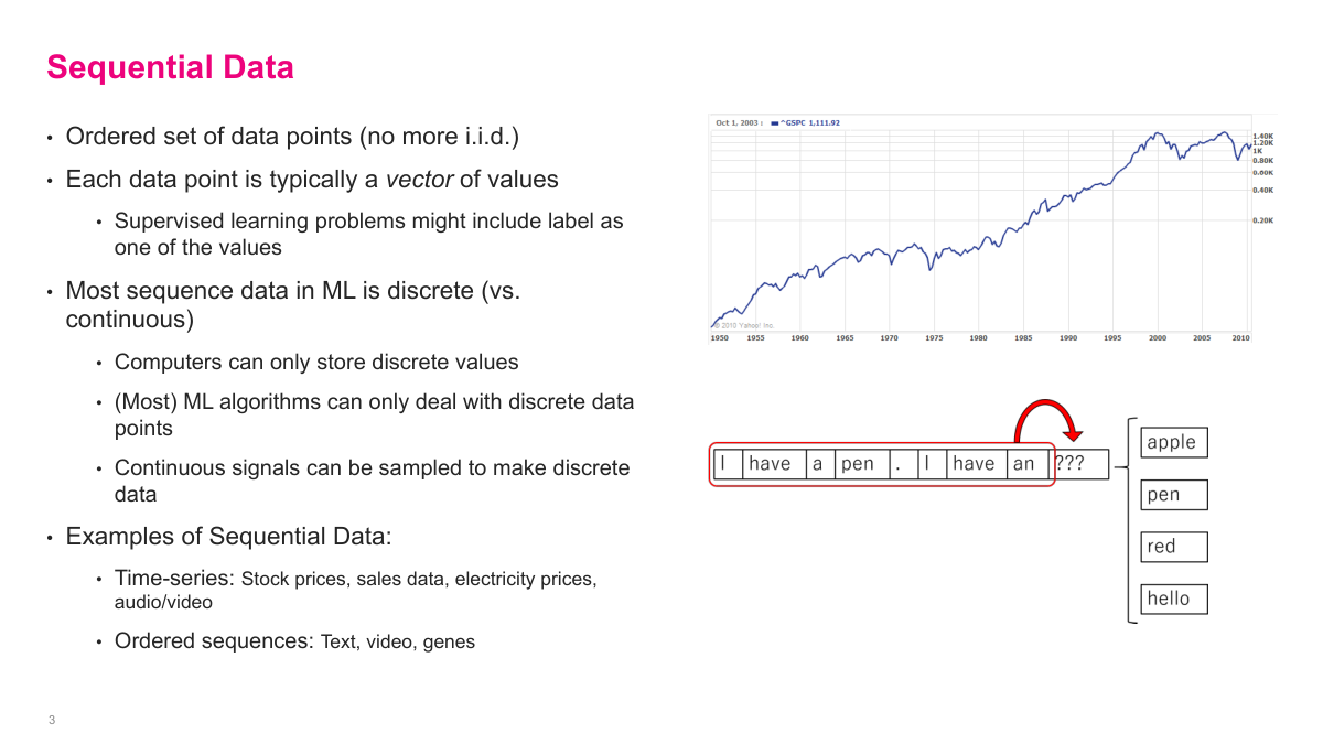
Sequential data is data where order matters, so the usual i.i.d. assumption breaks down. I usually think of each step as a vector of values, observed in some meaningful order. In practice, most machine learning systems work with discrete samples rather than truly continuous signals, so even things like audio or time become sampled sequences. Time series, text, video, and genomic data all fit this pattern. The common problem is that the current item is usually related to what came before it, and I need a model that can represent that dependence.

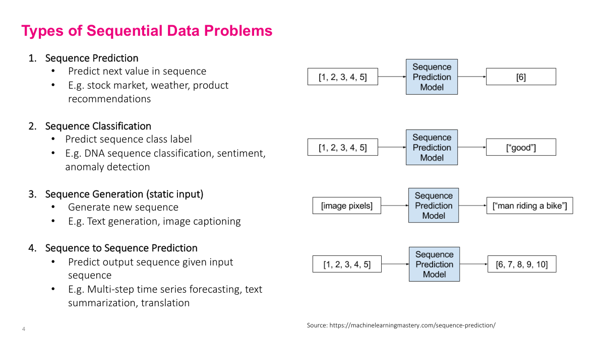
I group sequential problems into four common types. Sequence prediction maps a history to the next value. Sequence classification maps a whole sequence to a label, such as sentiment or anomaly detection. Sequence generation starts from some input and produces a sequence, as in image captioning. Sequence-to-sequence problems take one sequence in and produce another sequence out, which is the pattern behind translation, summarization, and many language-model tasks. This taxonomy is not exhaustive, but it covers most of the important cases.

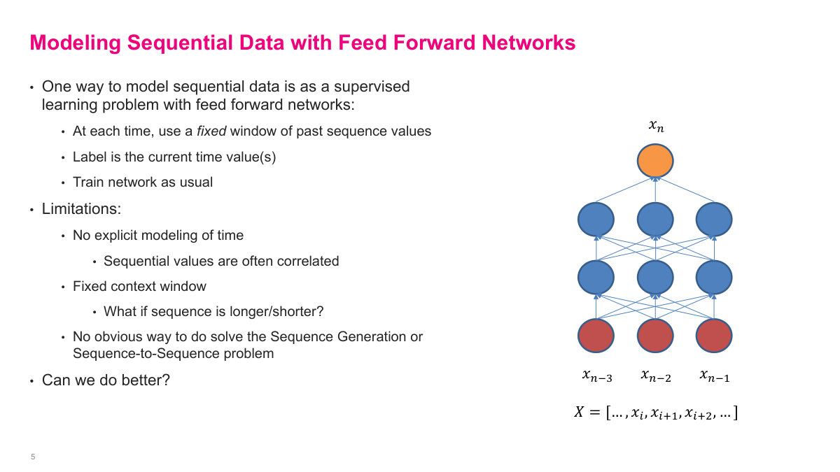
A simple baseline is to turn a sequence into a fixed-window supervised learning problem. I can feed x_{n-3}, x_{n-2}, and x_{n-1} into a standard feed forward network and ask it to predict x_n. That works, but it is crude. I have to choose the context window in advance, the model does not explicitly represent temporal structure, and it does not naturally handle generation or sequence-to-sequence tasks. This is exactly the gap recurrent networks are meant to close.

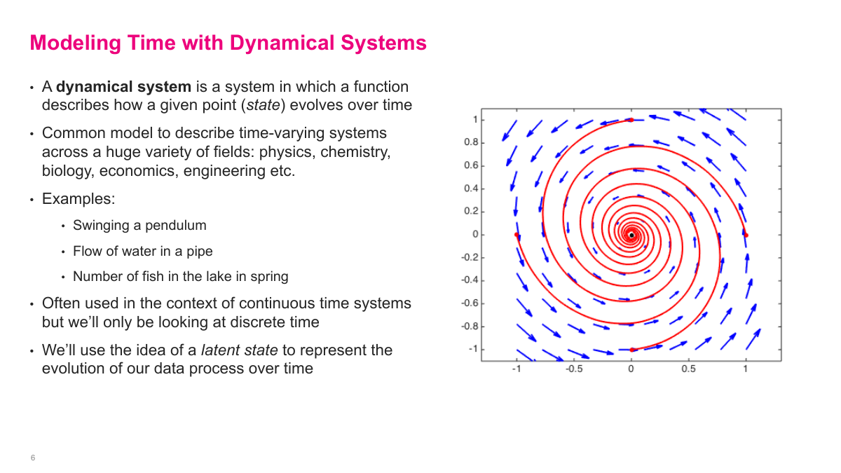
I use dynamical systems as the conceptual bridge to recurrent networks. A dynamical system describes how a state evolves over time according to a transition function. That framing shows up everywhere: physics, biology, engineering, economics. In machine learning, I usually care about the discrete-time version, where I observe a system at successive steps rather than continuously. The important extra idea is latent state: even if I cannot observe everything I need directly, I can introduce a hidden representation that summarizes the system and helps me model its evolution.

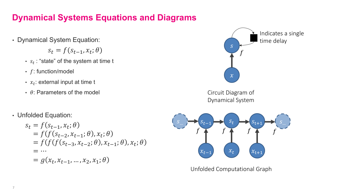
The key equation is s_t = f(s_{t-1}, x_t; θ). The same transition function takes the previous state and current input and produces the next state. If I unroll that recursion, the current state becomes a function of the whole input history. That is the exact mental model I want for recurrent networks: not a different computation at every step, but one learned function applied repeatedly over time. The diagrams on this slide make that concrete by showing both the compact recurrent view and the unfolded computational graph.

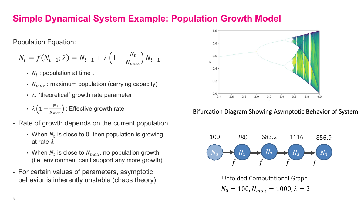
This fish-population example makes repeated state updates concrete. The population changes according to a growth rule that depends on the current population, the growth rate, and the carrying capacity. Early on, growth is fast. As the population approaches the limit, growth slows or reverses. What matters here is not the biology so much as the structure: I keep applying the same function to the current state and watching the trajectory evolve. It also shows an important warning sign for recurrent models: repeated function application can become highly sensitive to initial conditions and can produce unstable behavior.

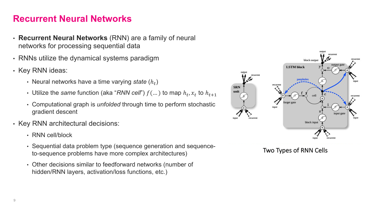
A recurrent neural network is a family of models for sequential data built around a time-varying hidden state. Instead of treating every input independently, I introduce a hidden state h_t that carries information forward. The same RNN cell is reused at every time step, so the model learns one transition rule rather than a separate computation for each position. I can then unfold that recurrence through time and train it with gradient-based methods. The main design choices are the cell itself, the problem setup, and the usual neural-network decisions around depth, activations, and outputs.

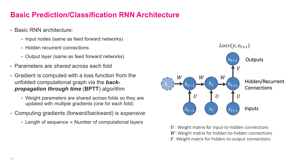
This is the standard unfolded RNN picture. Inputs feed into hidden states, hidden states connect across time, and an output layer can sit on top of the hidden representation. The key detail is parameter sharing: the same U, W, and V matrices are used at every fold. That gives the model its recurrent structure and keeps the number of learned parameters manageable. Training works by back-propagation through time, which is just gradient descent on the unfolded computational graph. The downside is that long sequences effectively create very deep graphs, so the computation becomes expensive and gradients become harder to manage.

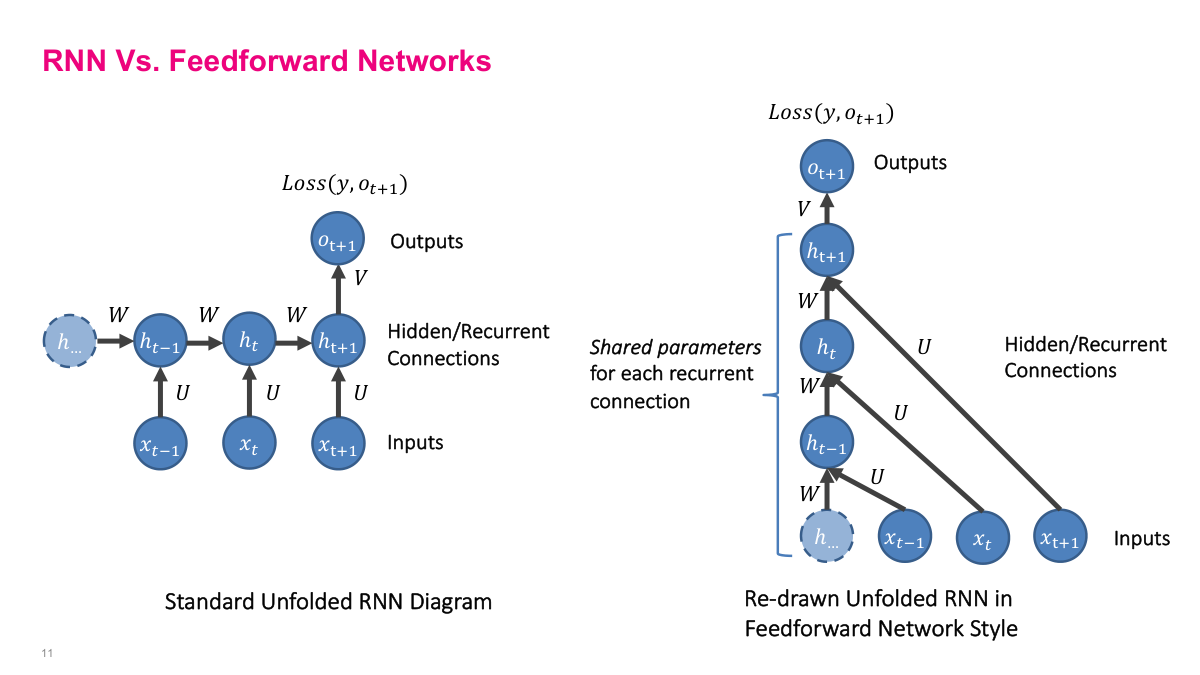
I like this slide because it strips away some of the mystery. An unfolded RNN can be redrawn to look a lot like a deep feedforward network. The difference is that the hidden-to-hidden transformation is reused across time instead of learning a different weight matrix at each layer. That shared structure is powerful because it lets me process variable-length sequences with one model, but it also creates the optimization problems that make simple recurrent networks difficult to train.

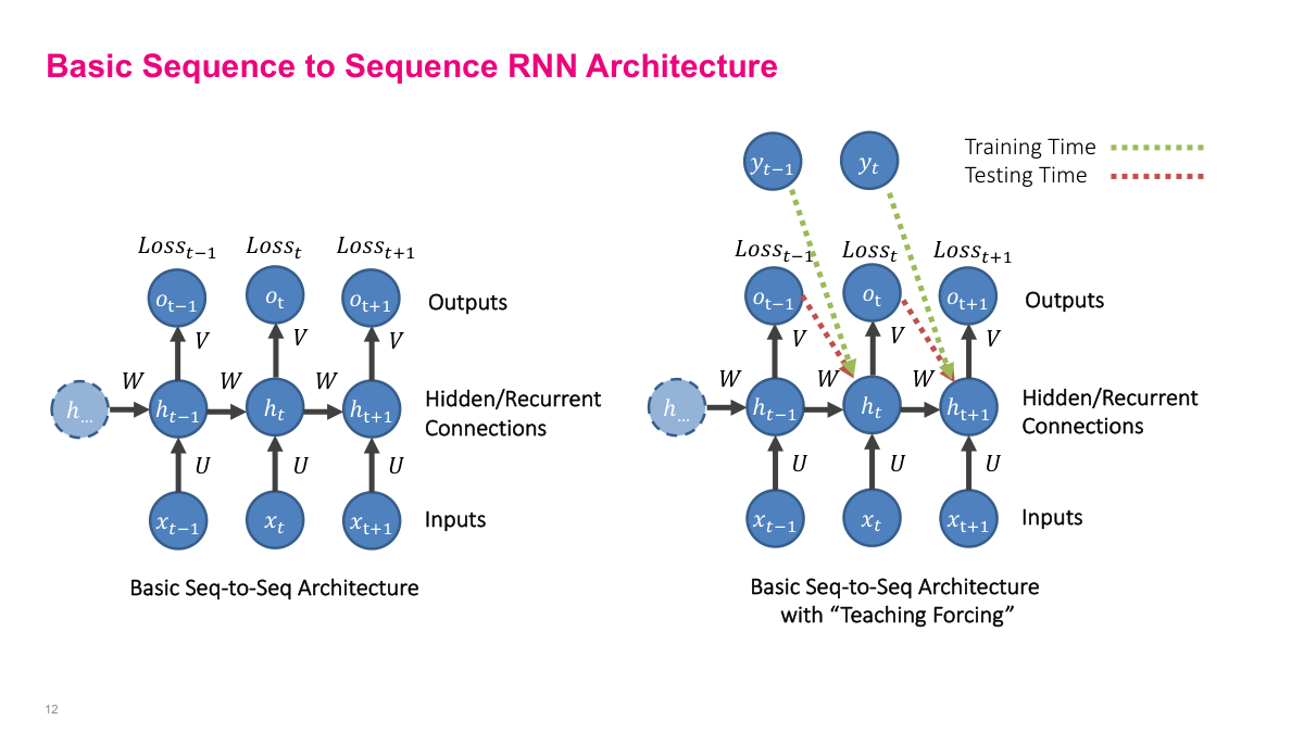
For sequence-to-sequence problems, I often want the model to predict the next item at every step. During training, I can compare each predicted output to the correct next token or next value and accumulate a loss across the whole sequence. Teacher forcing makes this easier by feeding the true previous output back into the model during training, rather than forcing the model to rely only on its own earlier predictions. At inference time, that support disappears and the model has to feed its generated outputs back into itself. This distinction between training-time and test-time behavior is one of the central practical details in sequence models.

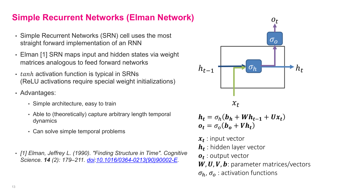
The Elman network is the simplest recurring cell: combine the previous hidden state and current input through learned weight matrices, apply a nonlinearity such as tanh, and optionally map the hidden state to an output. Conceptually, it is just a straightforward extension of a feedforward network. The appealing part is its simplicity. I only need one recurrent state, the same transition is used at every step, and the whole model is still differentiable end to end. The problem is that this elegance does not translate into robustness. In practice, simple recurrent networks are easy to write down but much harder to train well on long or complex sequences.

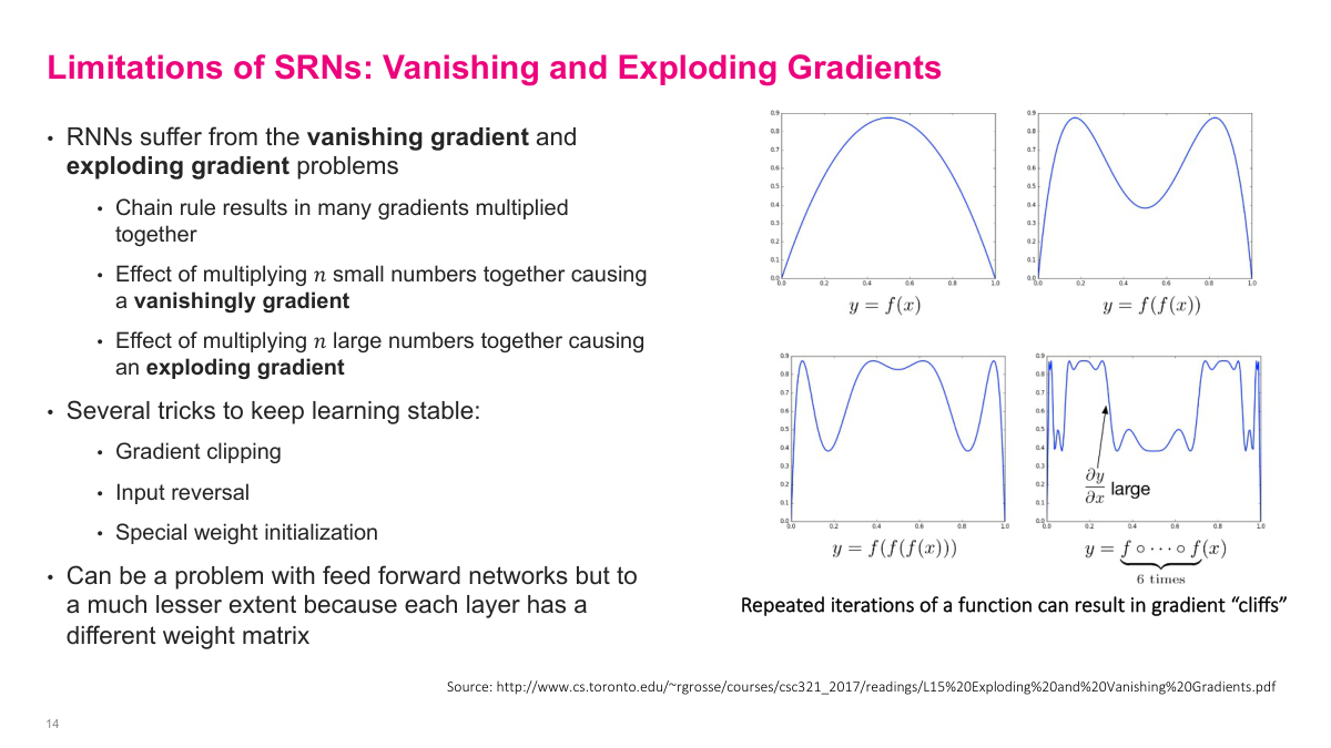
Simple recurrent networks suffer badly from vanishing and exploding gradients. When I back-propagate through many time steps, I end up multiplying many derivatives together. If those factors are mostly small, the gradient shrinks toward zero and early time steps stop learning. If they are mostly large, the gradient can blow up and training becomes unstable. There are mitigation tricks such as gradient clipping and careful initialization, but they do not fundamentally remove the issue. This is one of the main reasons more structured recurrent cells became necessary.

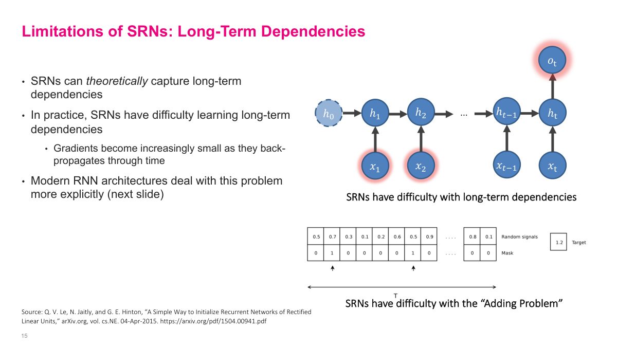
Even when a simple recurrent network should be able to represent a long-range dependency in theory, learning it in practice is difficult. Information from far back in the sequence has to survive many recurrent transitions, and gradients have to travel back through all of them. The adding problem on this slide is deliberately simple, but it exposes the weakness clearly: the model must remember just a few relevant positions over a long span and ignore everything else. That kind of selective memory is exactly where plain SRNs tend to fail.

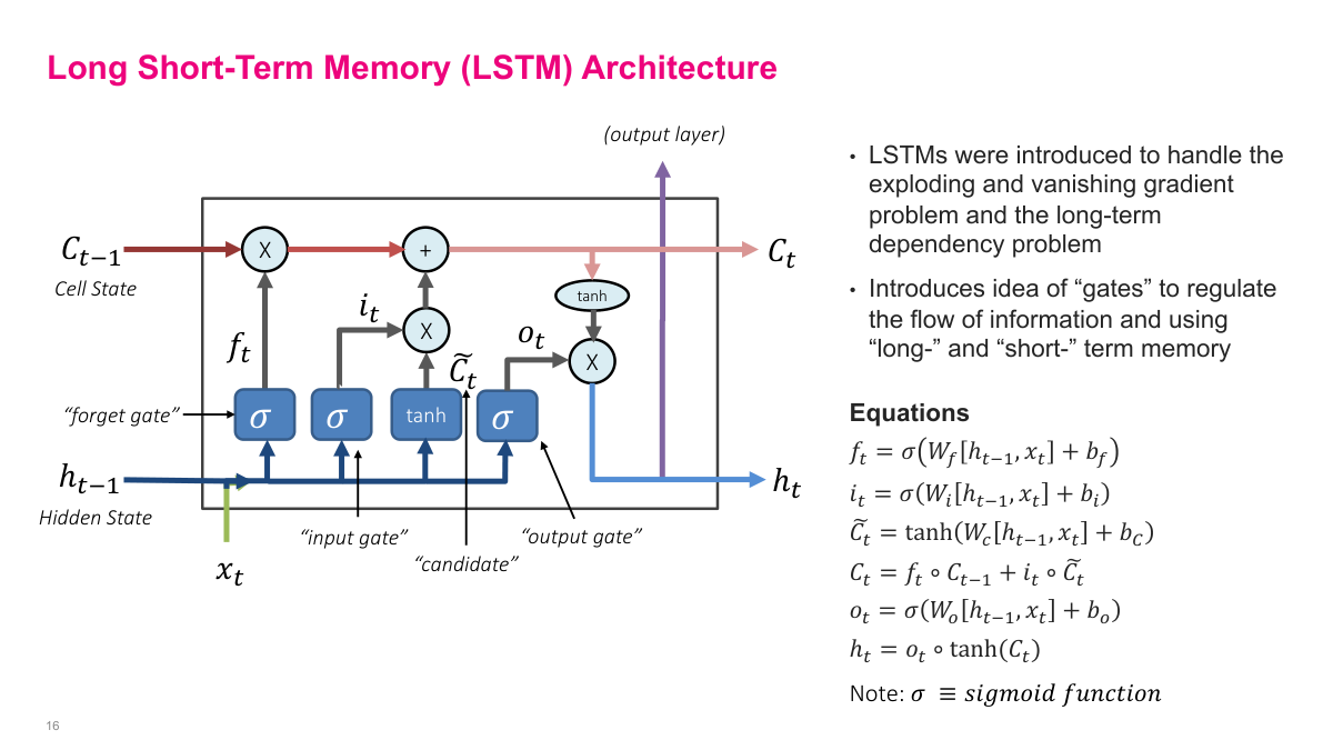
LSTMs were designed to address the weaknesses of simple recurrent networks. The core change is that I split the recurrent state into a cell state and a hidden state, then use gates to regulate how information flows. The forget gate decides what to discard, the input gate and candidate decide what to write, and the output gate decides what to expose as the next hidden state. The architecture is more complex than an SRN, but that extra structure is precisely what makes it much easier to preserve useful information over longer spans.

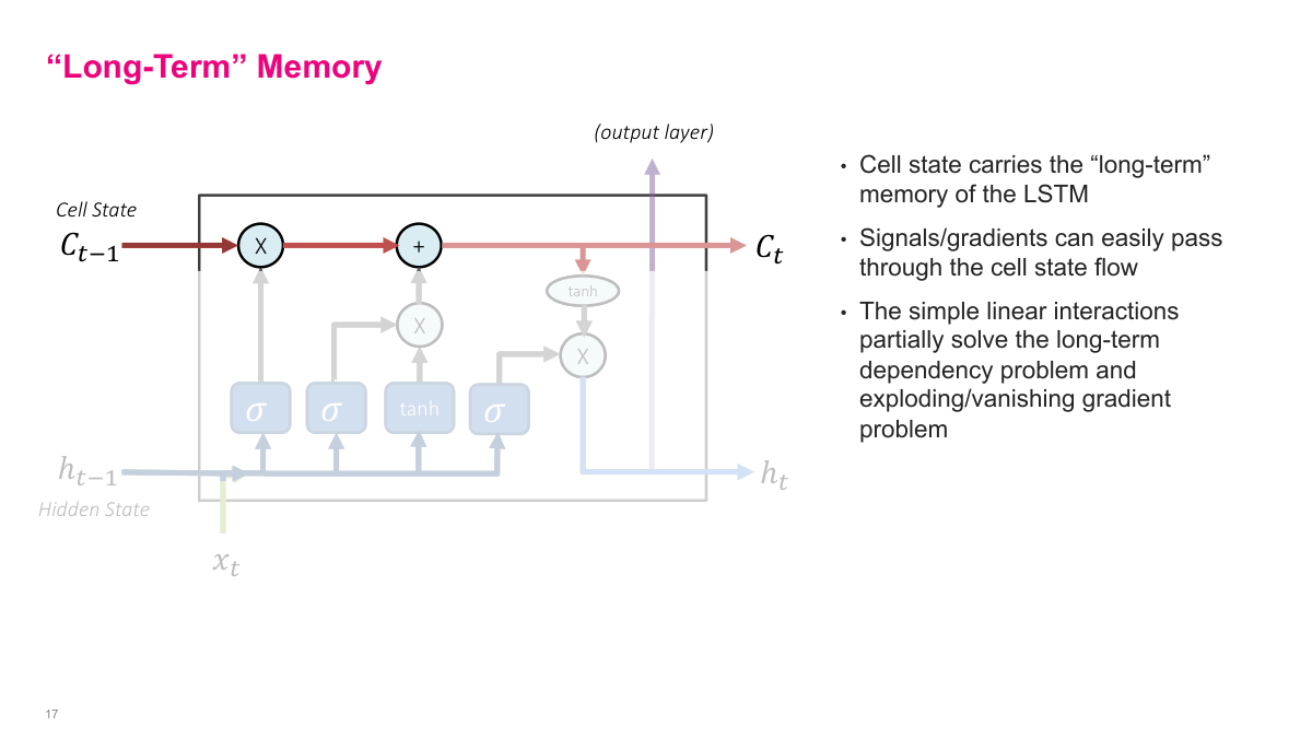
The cell state is the long-term memory path in an LSTM. I can think of it as the main highway carrying information across time, while the hidden state acts more like short-term working memory. Because the cell-state update is dominated by simple elementwise multiplication and addition, signals and gradients can pass through it more easily than in a plain recurrent cell. That is the core mechanism behind LSTM stability: it creates a path where information does not have to be repeatedly rewritten from scratch at every step.

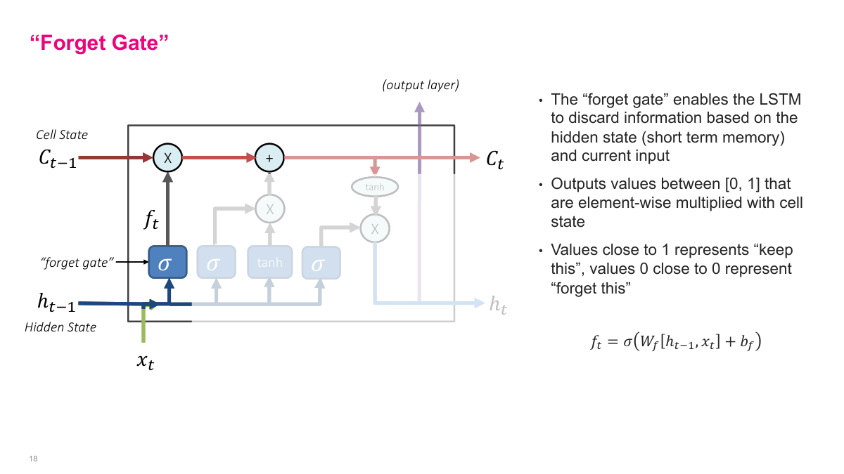
The forget gate gives the model a controlled way to erase information. It produces a vector of values between 0 and 1, one per dimension of the cell state, and multiplies them elementwise with the existing memory. Values near 1 keep the information, while values near 0 suppress it. I like to think of this as learned damping rather than literal deletion. The model decides, from the current input and prior hidden state, which parts of its memory are still useful and which parts should fade away.

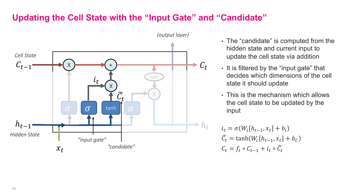
The input gate and candidate work together to write new information into memory. The candidate proposes content that might be useful, and the input gate decides how much of that proposal should actually enter the cell state. The update is additive: part of the old memory is preserved through the forget gate, and part of the proposed new content is added in. That combination is important. It means I can retain old information, overwrite only what matters, and make memory updates in a controlled, dimension-by-dimension way.

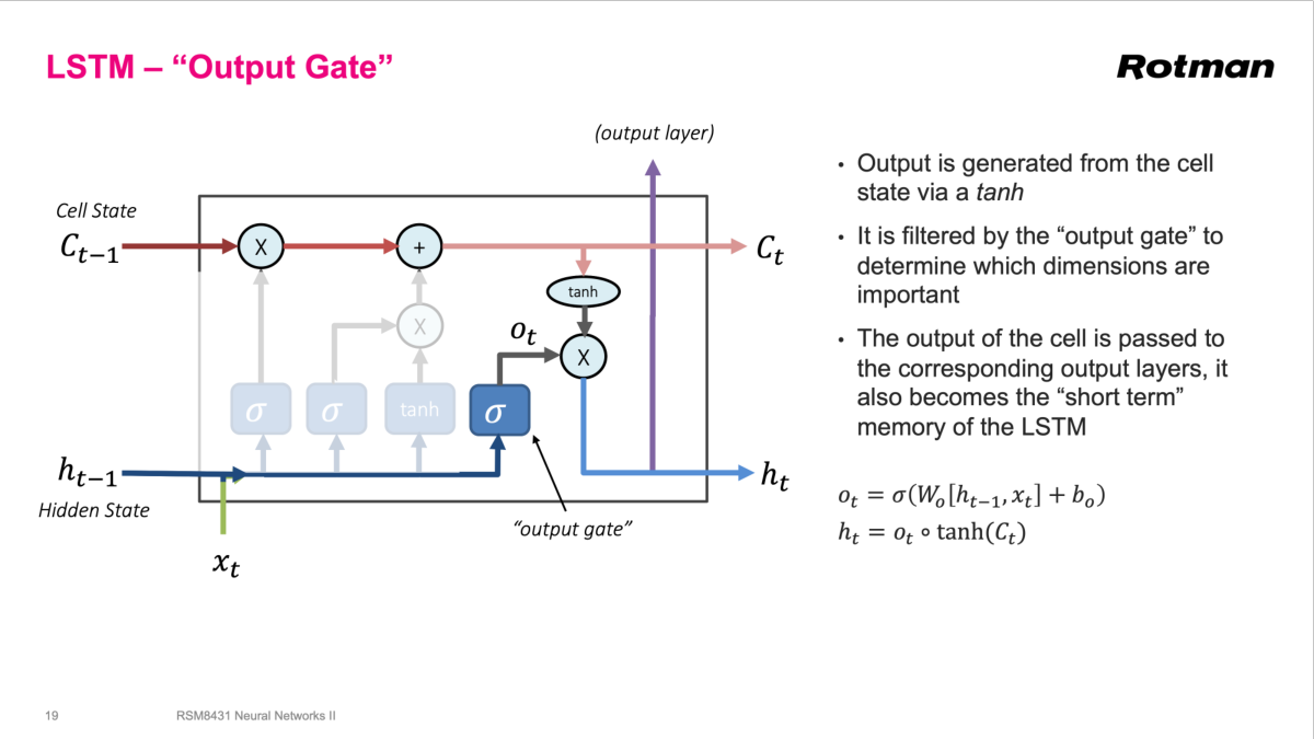
Once the cell state has been updated, the output gate decides what part of that internal memory should become visible as the next hidden state. The cell state passes through a tanh nonlinearity, then the output gate filters it elementwise. This hidden state serves two purposes at once: it is the short-term state passed to the next recurrent step, and it is the representation I can feed to downstream output layers. In other words, the output gate controls what the LSTM says externally, not just what it remembers internally.

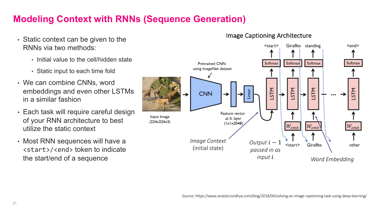
RNNs do not have to start from an empty context. I can inject static context either through the initial hidden state or as a repeated conditioning input at each time step. Image captioning is a good example: a pretrained CNN extracts an image representation, that representation initializes the recurrent model, and the LSTM generates words one by one until it emits an end token. The special start and end tokens matter because the model needs explicit markers for when generation begins and when it should stop.

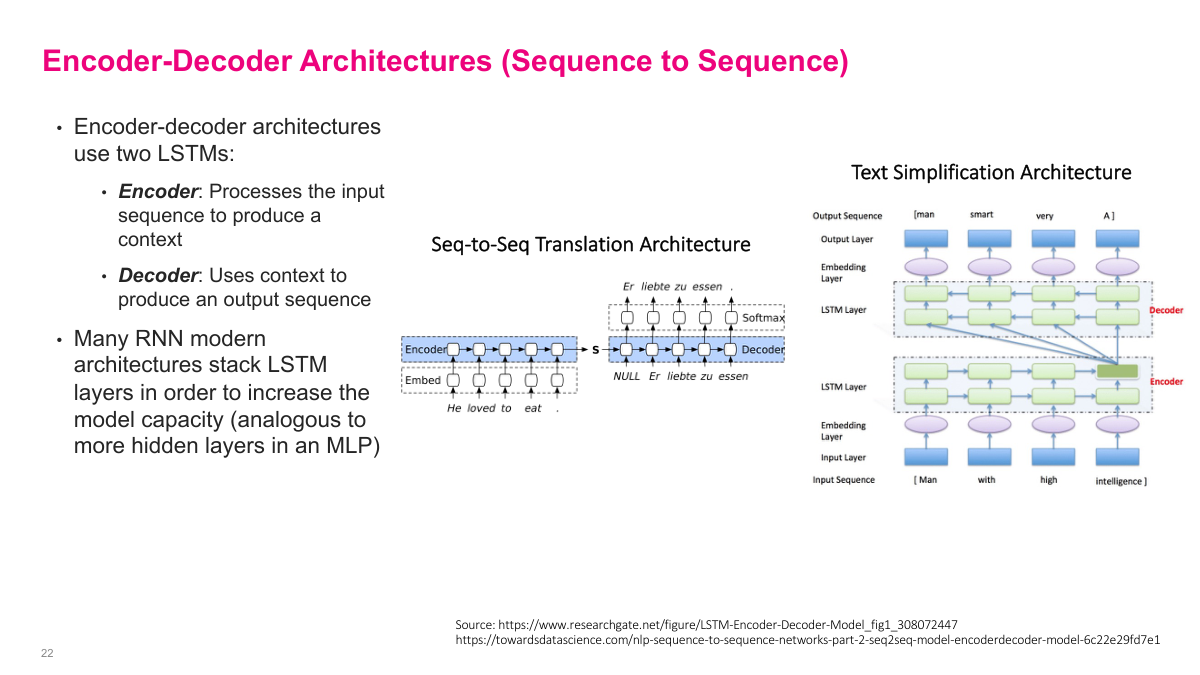
Encoder-decoder models split the sequence problem into two stages. The encoder reads the full input sequence and compresses it into a context representation. The decoder then uses that representation to generate the output sequence. This pattern is especially natural for translation, where I often need to read the entire source sentence before I can produce a fluent target sentence. The slide also shows stacked LSTM layers, which are the recurrent analogue of adding more hidden layers in a multilayer perceptron: they increase capacity and let the model learn richer intermediate representations.

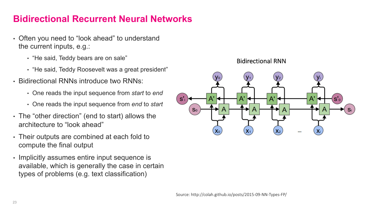
A bidirectional RNN processes the same sequence in two directions: one recurrent network reads from start to end, and another reads from end to start. I then combine their outputs at each position. This matters when future context helps interpret the current token. The teddy-bears versus Teddy-Roosevelt example makes the point well: the meaning of an early word can depend on what comes later. Bidirectional models are therefore especially useful when the full input sequence is available up front, as in many classification and tagging problems.

The review closes the loop on the five opening questions. The four major sequential problem types are prediction, classification, generation, and sequence-to-sequence mapping. An RNN is a model that processes ordered inputs by repeatedly applying the same transition function to a hidden state. Simple recurrent networks suffer from vanishing and exploding gradients and struggle with long-term dependencies. LSTMs address those problems by adding a structured memory system built around a cell state plus forget, input, and output gates.

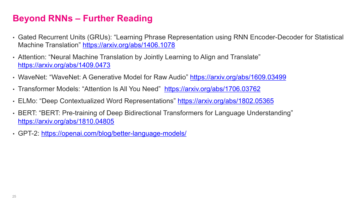
This slide points to the lineage that extends beyond classical RNNs. GRUs simplify the LSTM idea while keeping gating. Attention relaxes the bottleneck of forcing everything through a single recurrent state. WaveNet shows how sequence modeling can be done in raw audio. Transformers ultimately became the dominant architecture for many sequence tasks, and models such as ELMo, BERT, and GPT-2 build directly on that shift. I think of this slide as the handoff from recurrent sequence modeling to the modern language-model era.