Lecture 05: CNN

This section covers convolutional neural networks from the ground up -- starting with the mathematical operation of convolution, building up to CNN architectures, and finishing with normalization techniques. We'll also touch on transfer learning and how pre-trained models can be leveraged for new tasks.

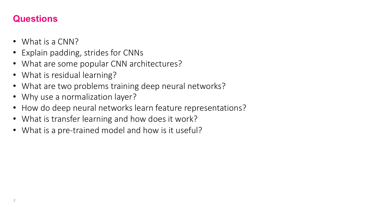
The key questions for this section: What is a CNN? Can you explain padding and strides? What are some popular CNN architectures? What is residual learning, and what two problems arise when training deep neural networks? Why use normalization layers? And on the transfer learning side -- what are learned feature representations, how does transfer learning work, what is a pre-trained model, and how is it useful?

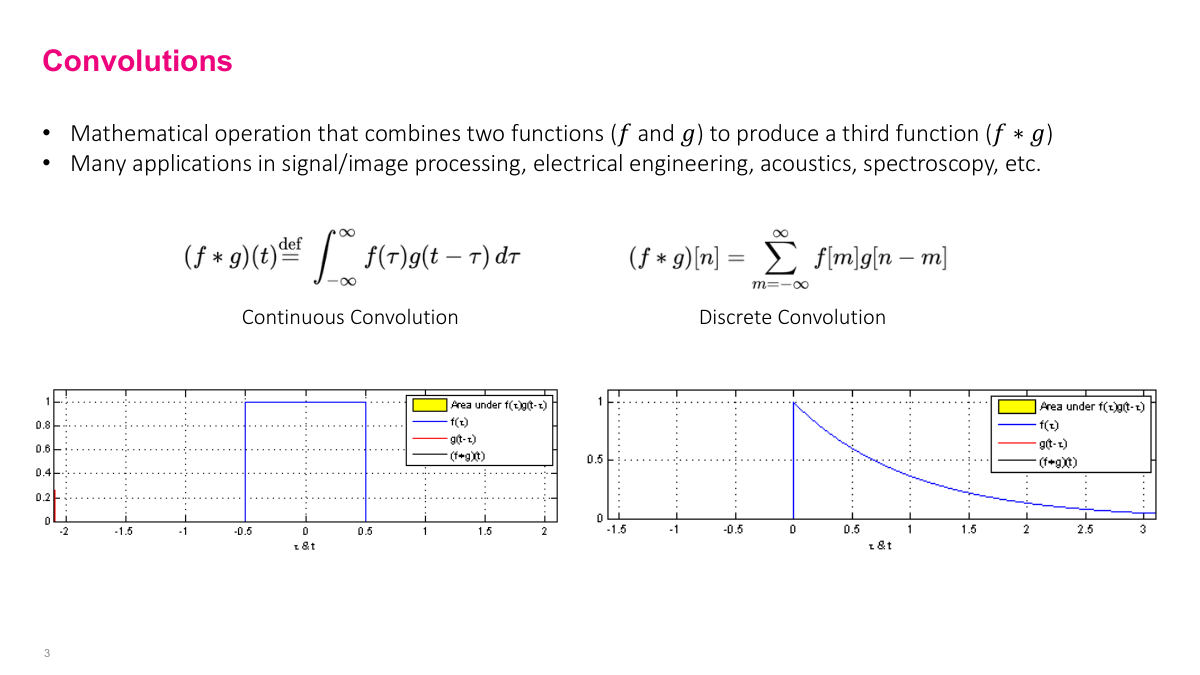
Convolution is a mathematical operator on two functions. In the continuous case it's an integral, in the discrete case it's a summation. Visually, you're taking one function and sliding it over the other from negative infinity to positive infinity, computing the overlap at each position. The diagrams here show two functions -- one is a rectangular pulse that's zero everywhere except for a fixed region. As you slide one function across the other, the output traces the convolution result. This is a foundational operation in signal processing, and it's the core building block of CNNs.

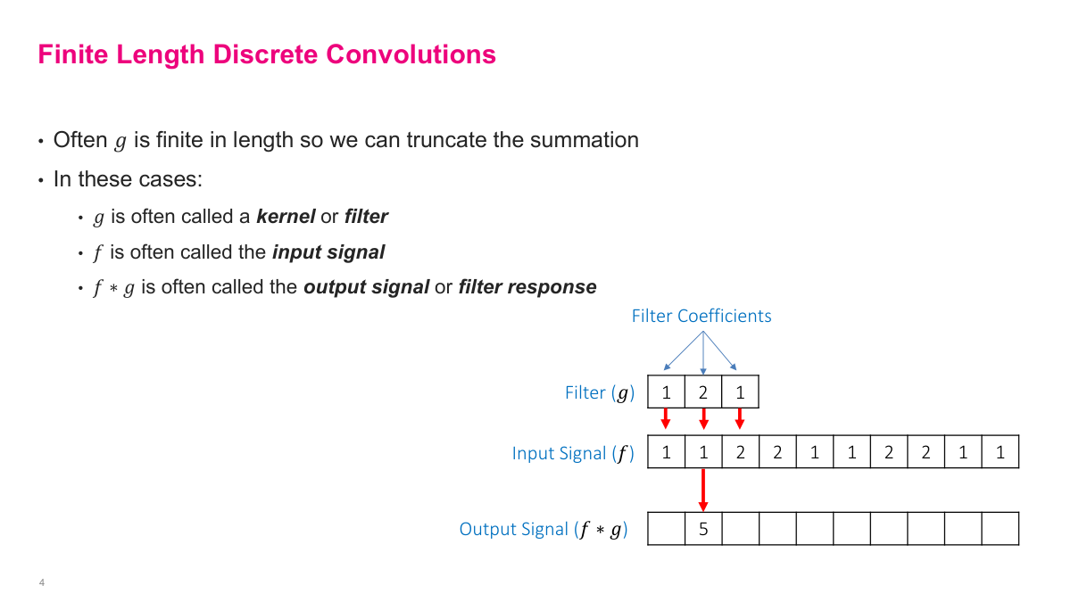
In practice, one of the functions is small and fixed in length -- this is called the kernel or filter. It's typically 3, 5, or 7 elements wide. The other function is the input signal, which in the context of CNNs is usually an image. You slide the kernel over the input, computing a dot product at each position, and the result is called the output signal or feature response. The diagram shows a filter [1, 2, 1] sliding over an input signal to produce the first output value. This finite, discrete version of convolution is what actually gets computed in neural networks.

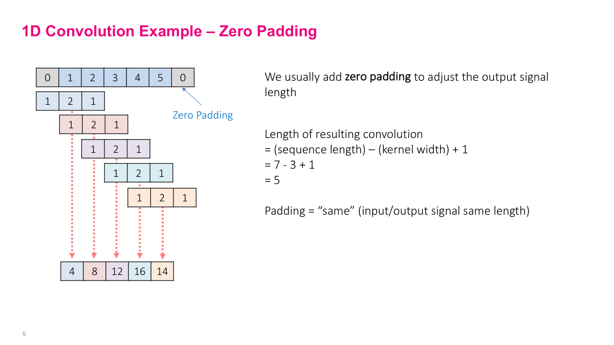
Here's a concrete 1D example. The filter is [1, 2, 1] and the input is [0, 1, 2, 3, 4, 5, 0] with zero padding on each end. At each position, you compute the dot product: 1 times 0, plus 2 times 1, plus 1 times 2 gives 4. Shift one step, and you get 1 times 1, plus 2 times 2, plus 1 times 3 which is 8. You keep sliding the window across the entire signal. The zeros on either end are "zero padding" -- they let the filter reach the edges of the input. With "same" padding, the output has the same length as the input. Without padding ("valid"), the output shrinks because the filter can't extend past the boundaries. The formula is: output length equals input length minus kernel width plus one.

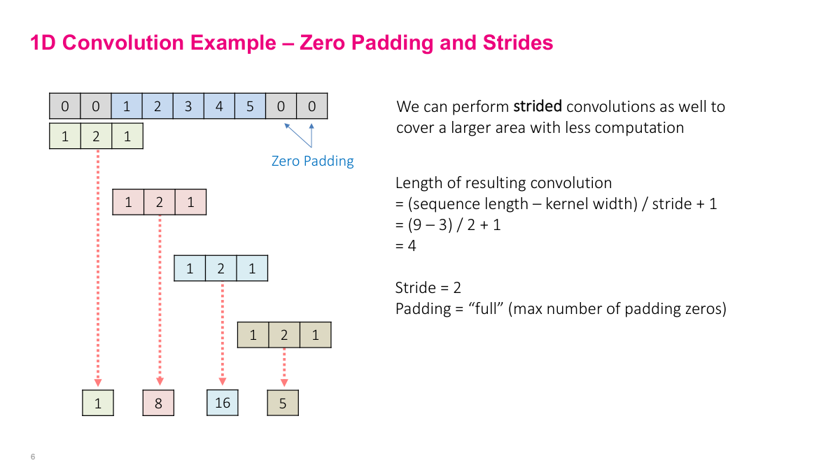
We don't have to move the filter one step at a time -- we can jump more than one position, and that's the idea of strides. A stride of 2 means we skip every other position, reducing the output length. This example also shows "full" padding, which is the maximum number of zeros you can add such that the filter still overlaps with at least one element of the input signal. Adding more zeros beyond that would just produce zeros in the output. Between padding and strides, you have two knobs that control the spatial dimensions of the output: padding preserves or increases the size, strides reduce it.

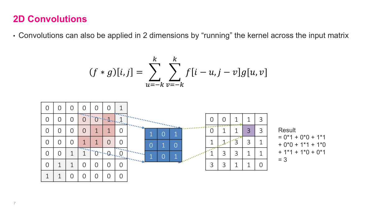
Images are two-dimensional, so we need 2D convolutions. The equation looks more complicated, but the idea is the same -- instead of sliding a 1D filter along a signal, we slide a 2D kernel across rows and columns. At each position, we compute the element-wise product of the kernel and the overlapping patch of the input, then sum everything up. The kernel here is a small grid of values (like ones and zeros), and we scan it across the full image in both dimensions to produce the output feature map.

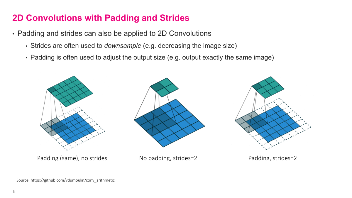
These visualizations show the effect of different padding and stride combinations on 2D convolutions. The bottom grid is the input, the shaded region is the filter, and the top grid is the output. With no padding and stride 1, the output shrinks. Adding "same" padding (one layer of zeros around the input) keeps the output the same size. Increasing the stride to 2 or 3 reduces the output dimensions further because the filter jumps multiple positions between computations. These two parameters -- padding and stride -- give you precise control over the spatial dimensions at each layer.

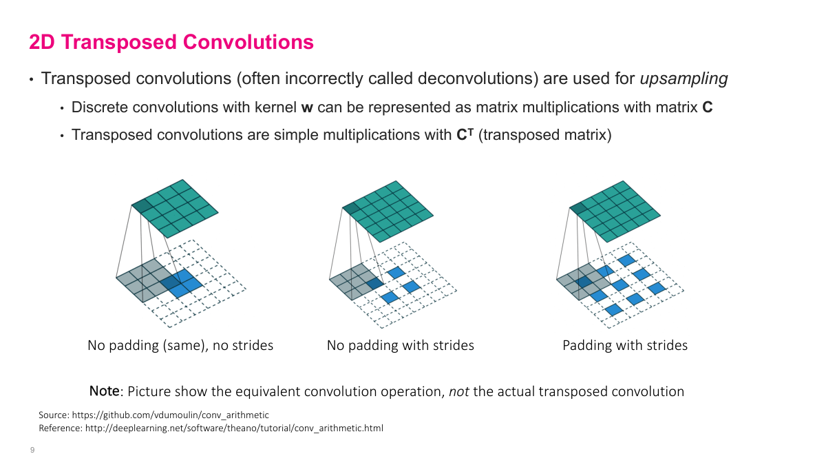
Transposed convolutions go in the opposite direction -- from a small input to a larger output. The blue is still the input, but now a 2x2 input can generate a larger output through this operation. The filter still exists (the shaded area), but it's applied in a way that upsamples rather than downsamples. This is useful in architectures that need to produce spatial outputs larger than their inputs, like image segmentation or generative models. While strides in regular convolutions reduce dimensions, transposed convolutions increase them. You'll sometimes hear these called "deconvolutions," though that's technically a misnomer.

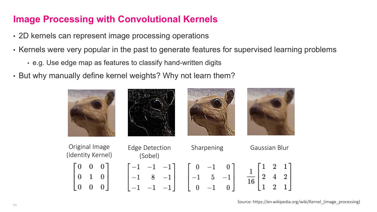
Before deep learning, people hand-designed convolutional kernels for image processing tasks. These kernels can perform edge detection, sharpening, blurring, and other operations depending on the weight values. For example, a Sobel kernel detects edges, a Gaussian kernel blurs, and a sharpening kernel enhances details. You might have used some of these in Photoshop. In the old days, these manually defined kernels were used to generate features for supervised learning -- for instance, using an edge map as input features to classify handwritten digits. But the obvious question is: why manually define kernel weights when we could learn them? That insight is the foundation of convolutional neural networks.

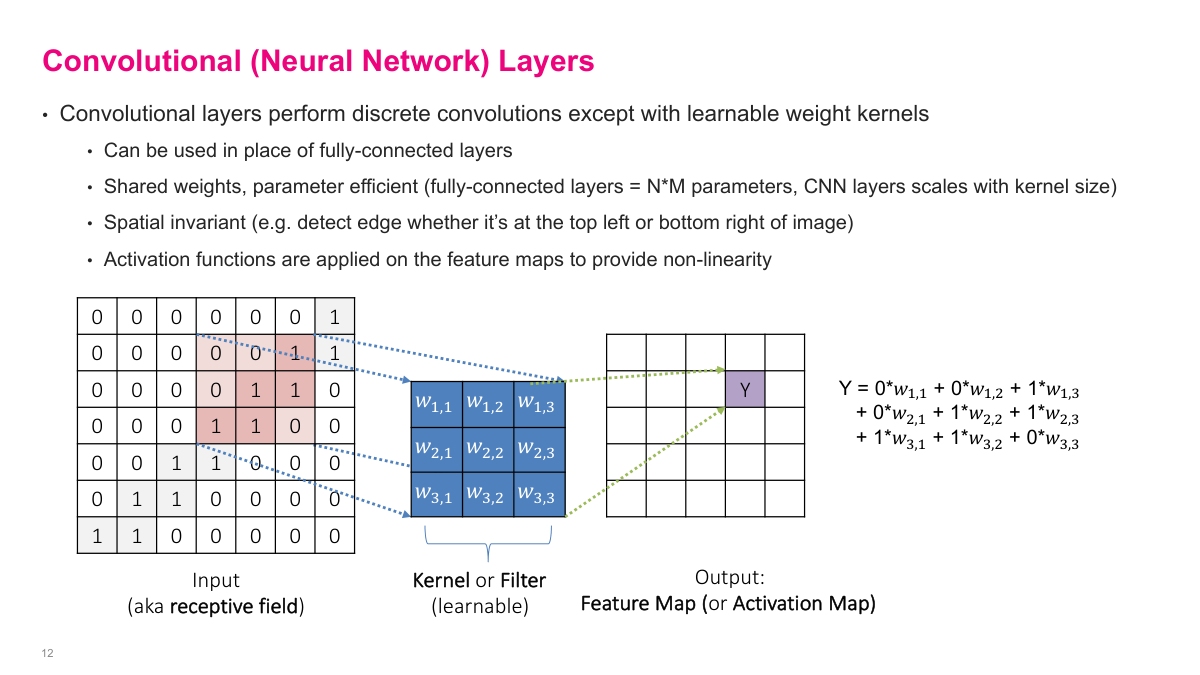
Instead of hand-picking kernel values, we replace them with learnable weights -- w1,1, w1,2, etc. The convolution operation is the same: take a 2D input, slide the kernel over it, and produce a feature map (also called an activation map). The key advantage is that convolutional layers share weights across all spatial positions, making them far more parameter-efficient than fully connected layers. They're also spatially invariant -- the same filter detects a pattern whether it appears in the top-left or bottom-right of the image. Activation functions are applied on the feature maps to provide non-linearity, just like in fully connected networks.

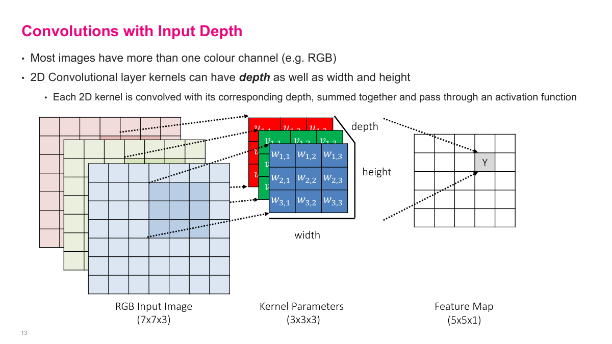
Real images aren't 2D -- they have depth. A color image has three channels (RGB: red, green, blue), so a 7x7 image is actually 7x7x3. The convolutional kernel must match this depth, so instead of a 3x3 filter, you have a 3x3x3 filter. The operation works the same way: slide the 3D kernel across the spatial dimensions, computing element-wise products across all three channels and summing everything into a single value. The output is still a 2D feature map because the depth dimension gets collapsed during the dot product. This is an important detail -- the kernel always spans the full depth of the input.

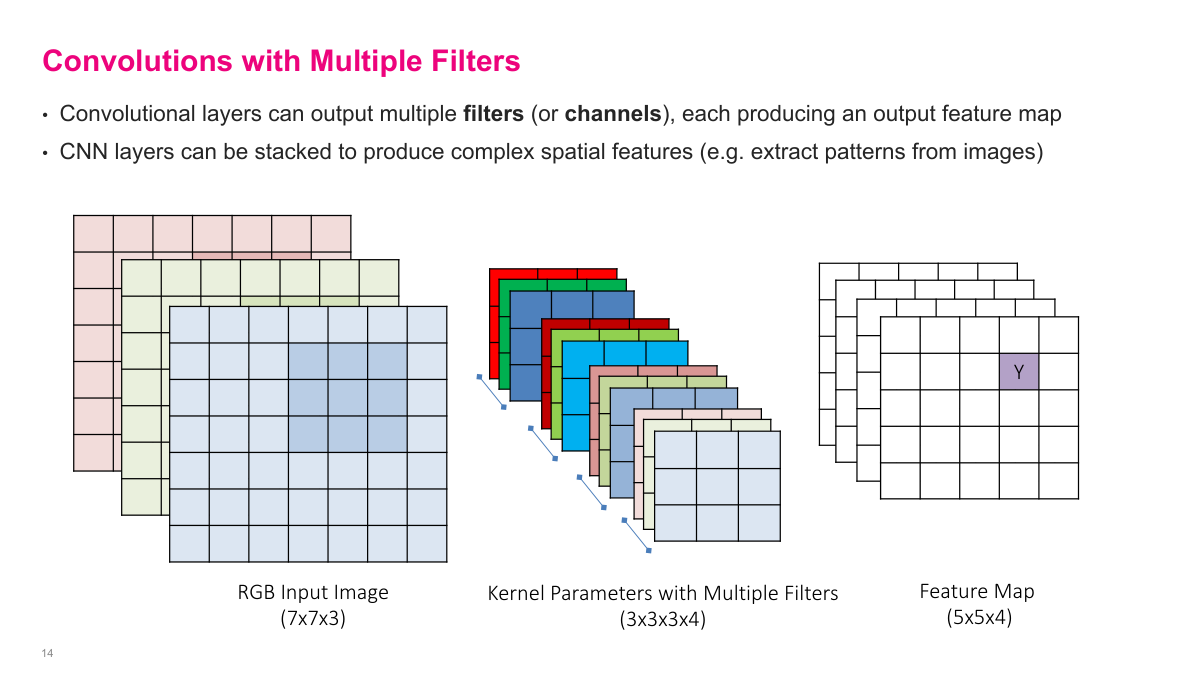
To capture multiple patterns, we use multiple filters. Each filter is a full 3D kernel (matching the input depth) and produces its own 2D feature map. If I have four filters, I get four feature maps stacked together as the output. Each filter operates independently on the same input, and each one learns to detect different patterns. The output depth equals the number of filters -- so a layer with 64 filters produces an output with depth 64. This is how convolutional layers build up rich representations: each filter specializes in a different feature.

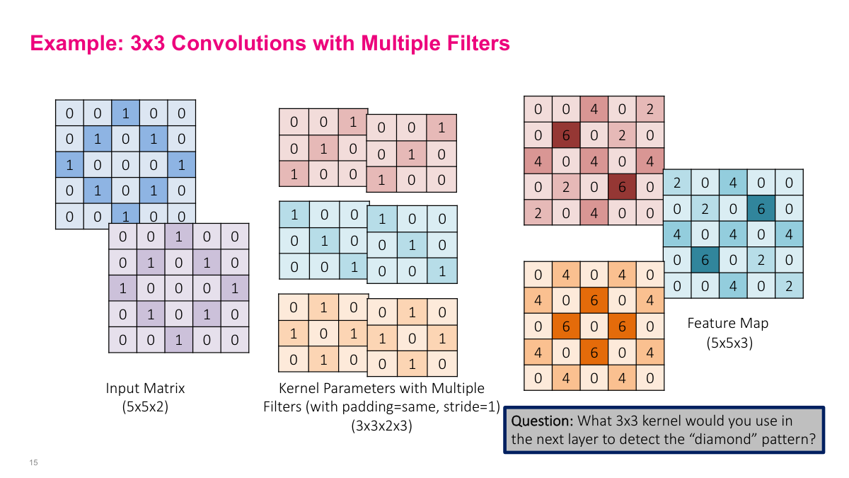
This example shows three 3x3 filters applied to a 5x5x2 input containing a diamond pattern. Each filter produces a different 5x5 feature map that highlights different aspects of the pattern. One filter detects diagonal lines going one way, another detects diagonals going the other way, and the third picks up the cross/plus pattern. The cells with the highest values (6 in the output) indicate the strongest pattern matches. The slide poses a good question: what 3x3 kernel would you use in the next layer to detect the full diamond pattern from these feature maps?

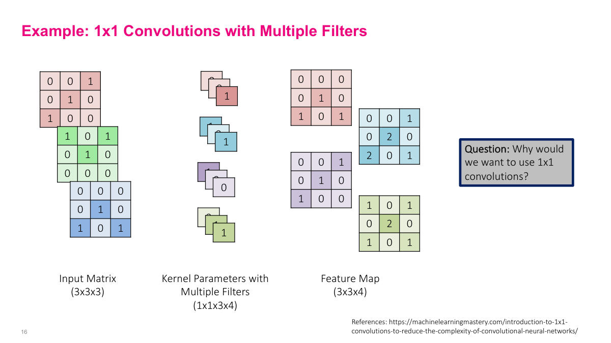
A 1x1 convolution is a special case that seems odd at first -- the spatial receptive field is just a single pixel, so it doesn't look at any surrounding pixels. But it operates across the full depth of the input. With a 1x1x3 kernel on an RGB input, it computes a weighted combination of the three color channels at each pixel location. If you have multiple 1x1 filters, each one learns a different linear combination of the input channels. This is essentially a per-pixel fully connected layer across the depth dimension. It's a common operation in CNN architectures because it lets you change the number of channels (increase or decrease depth) without changing spatial dimensions, and it's computationally cheap.

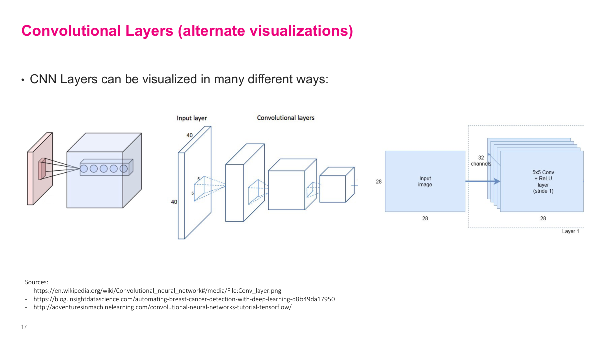
When dealing with multi-dimensional inputs and outputs, it helps to see different visual representations. These diagrams show the same convolutional operation from different perspectives -- the input volume, the kernel sliding across it, and the resulting output volume. One common representation shows the depth, height, and width as a 3D block, with a slice representing the kernel's operation. Another shows each layer's dimensions explicitly (like "40x40, 64 channels"). These visualizations are useful for understanding how dimensions flow through a network.

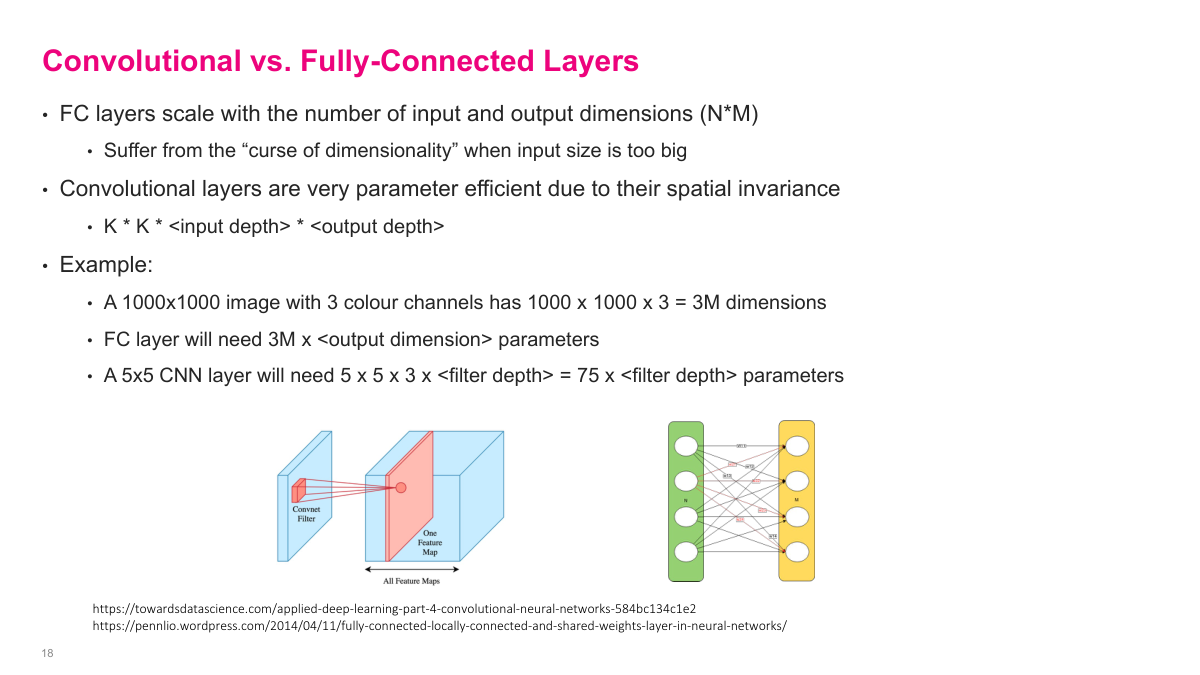
Fully connected layers scale with the number of input and output dimensions (N times M parameters), which suffers from the curse of dimensionality. A 1000x1000 image with 3 color channels has 3 million input dimensions -- a fully connected layer would need 3M times the output dimension in parameters. Convolutional layers are far more efficient because of spatial invariance: the parameter count is just kernel size times input depth times output depth. A 5x5 CNN layer on the same image only needs 5x5x3 times the filter depth = 75 times filter depth parameters. This massive reduction in parameters through weight sharing is what makes CNNs practical for image data.

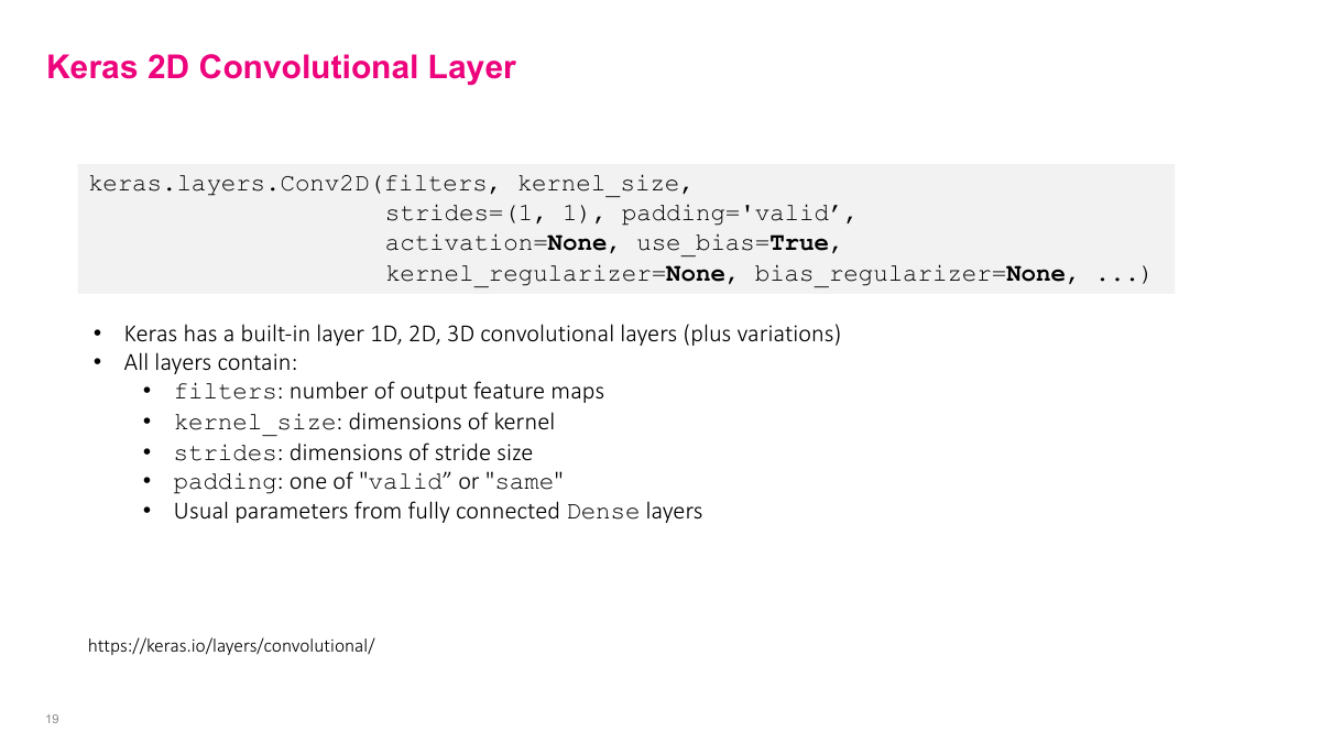
In Keras, the Conv2D layer exposes all the parameters we've discussed. filters sets the number of output feature maps. kernel_size can be a single number (assumed square, e.g., 3 means 3x3) or a tuple for non-square kernels. strides controls the step size in each dimension. padding can be "valid" (no padding) or "same" (pad to keep input and output spatial dimensions equal). You also specify the activation function and whether to include a bias term -- the standard configuration options for any neural network layer.

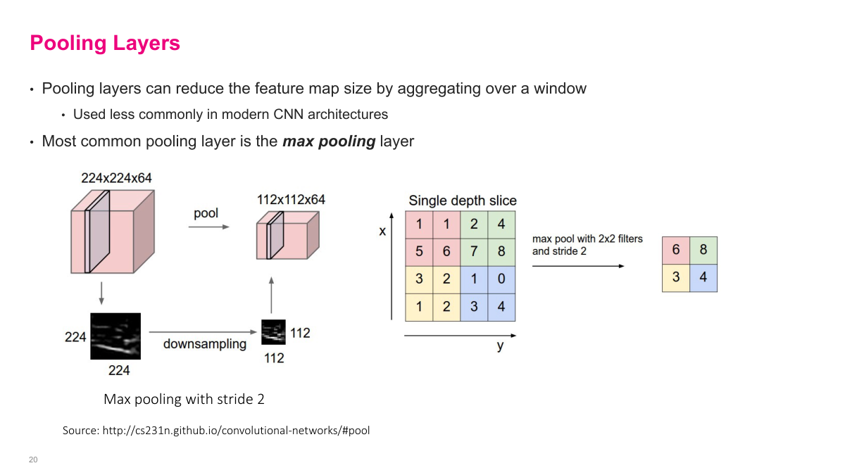
Pooling is another way to reduce spatial dimensions, separate from using strides. The most common form is 2x2 max pooling: partition the feature map into non-overlapping 2x2 blocks and take the maximum value from each block. This halves both the height and width. Average pooling takes the mean instead. Pooling was very popular in early CNN architectures as the primary way to downsample, though modern networks often prefer strided convolutions instead. The key benefit of pooling is that it introduces a small amount of translation invariance -- shifting the input by a pixel or two often doesn't change the pooled output.

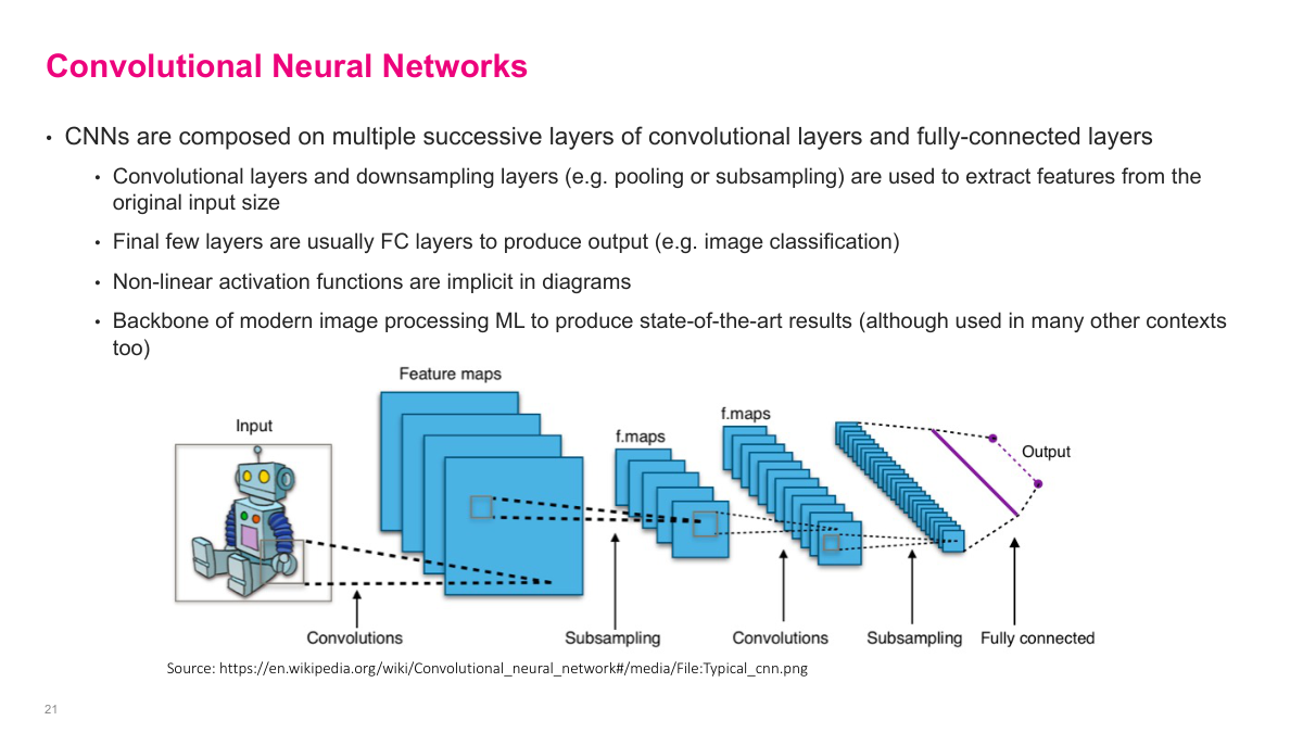
A CNN is built from different types of layers stacked together. You typically have convolutional layers, pooling or subsampling layers, and then fully connected layers near the end. The convolutional layers extract spatial features, pooling reduces dimensions, and the fully connected layers perform the final classification or regression. We're going to look at several historically important architectures that represent major milestones in CNN design and performance.

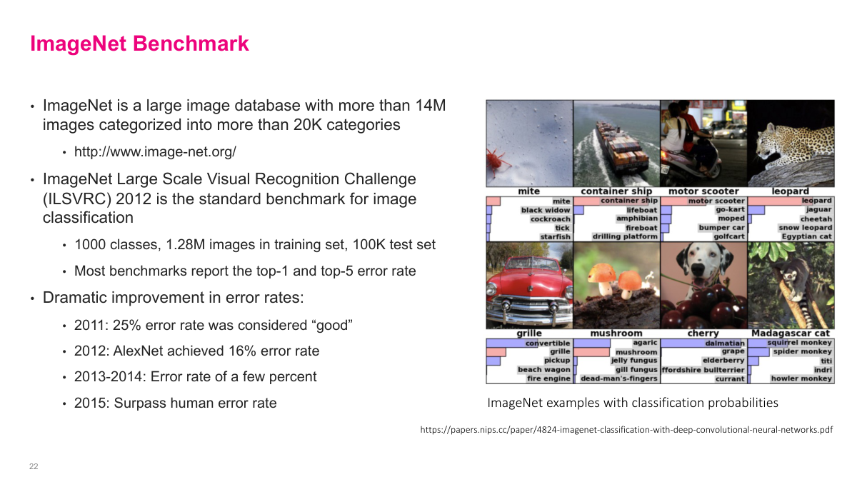
ImageNet is a massive image database with over 14 million images across more than 20,000 categories. It became the standard benchmark for evaluating image classification models. Given an image, the model outputs probabilities for each of the 1,000 classes. The benchmark uses "top-5 error rate" -- the model gets credit if the correct class appears in its five highest-probability predictions. ImageNet drove much of the progress in CNN architectures, with each year's competition winner introducing new ideas that advanced the field.

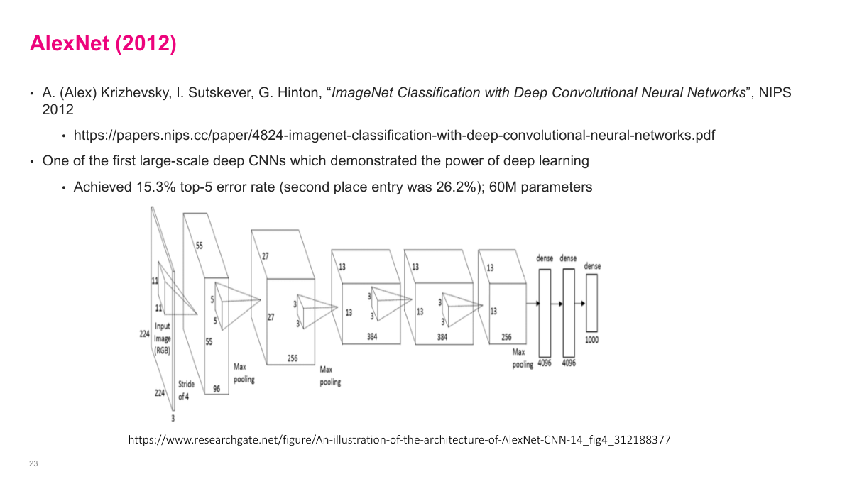
AlexNet was the breakthrough moment for deep learning. In 2012, it crushed the previous best results on ImageNet with an error rate around 15% -- a massive improvement over traditional computer vision methods. The team wrote low-level GPU code from scratch, including gradient computations, which was a huge engineering effort at the time. This is often called the "ImageNet moment" -- the point where the broader community realized neural networks were genuinely powerful. AlexNet used ReLU activations, dropout for regularization, and was trained on GPUs. It demonstrated that deep convolutional networks, with enough data and compute, could dramatically outperform hand-engineered features.

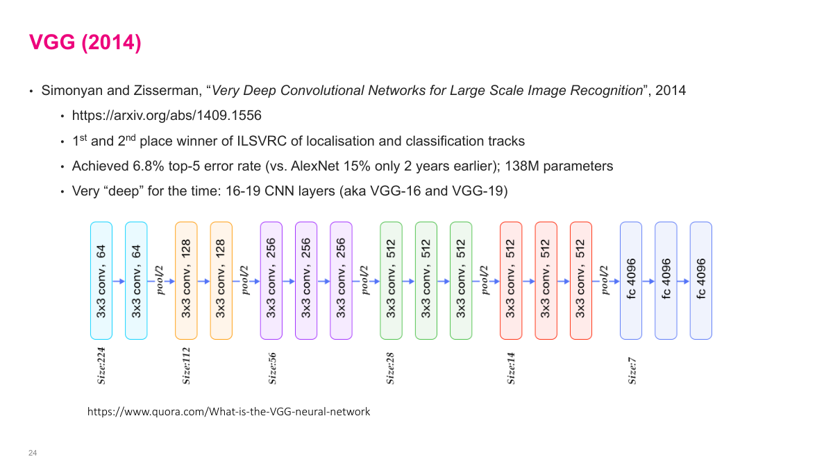
VGG won ImageNet in 2013-2014 with a top-5 error rate of 6.8%. It had 138 million parameters, which was large for its time. The key design principle was simplicity: just stack 3x3 convolutions and 2x2 max pooling repeatedly, increasing the number of feature maps as you go deeper. The architecture has 16-19 layers depending on the variant. VGG showed that depth matters -- using many small 3x3 filters is more effective than fewer large filters, while keeping the parameter count manageable. The architecture diagram shows the pattern clearly: convolution blocks followed by pooling, with increasing depth at each stage.

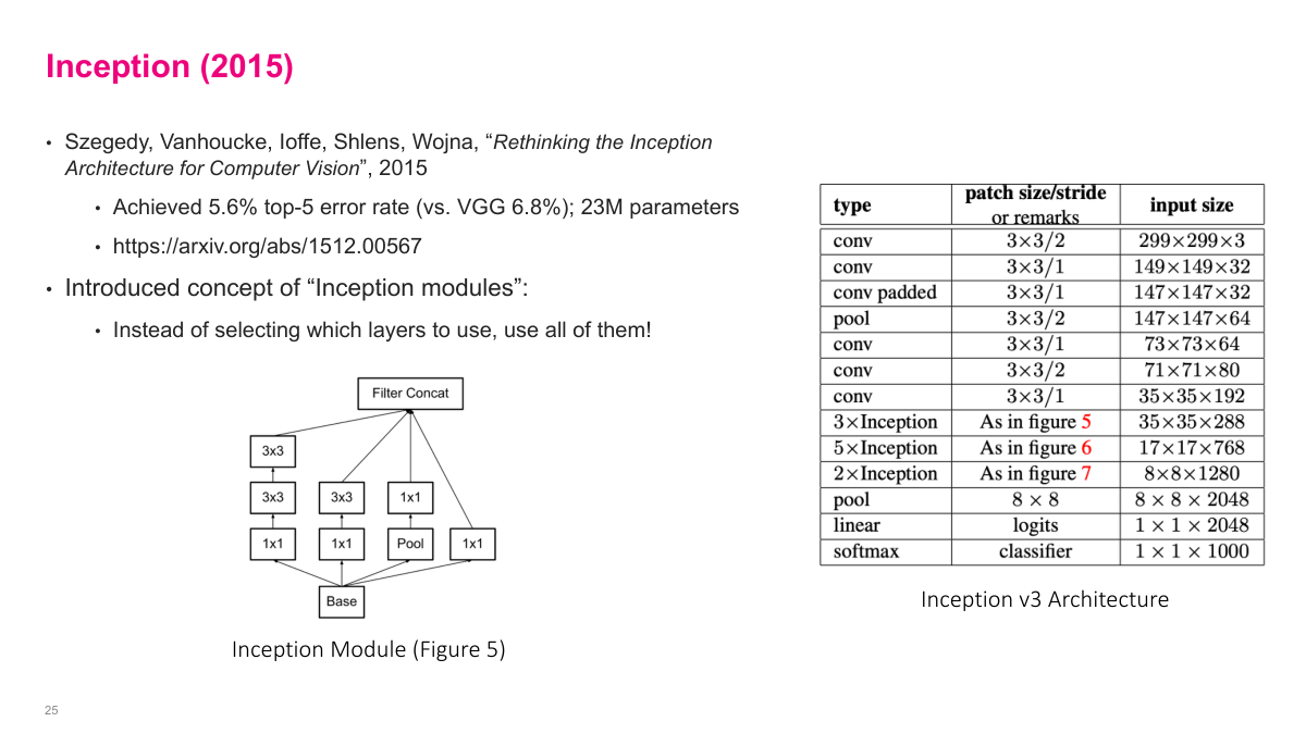
Inception achieved an even lower top-5 error rate of 5.6% with a creative architectural idea. Instead of choosing between 1x1, 3x3, or 5x5 convolutions, Inception uses all of them in parallel within a single module. The input flows into multiple branches -- a 1x1 convolution, a 3x3, a 5x5, and a max pooling path -- and the results are concatenated along the depth dimension. This "inception module" lets the network learn which filter sizes are most useful at each layer rather than the designer making that choice. To keep computation manageable, 1x1 convolutions are used as bottleneck layers to reduce depth before the larger convolutions. This was the beginning of more sophisticated, modular architecture design.

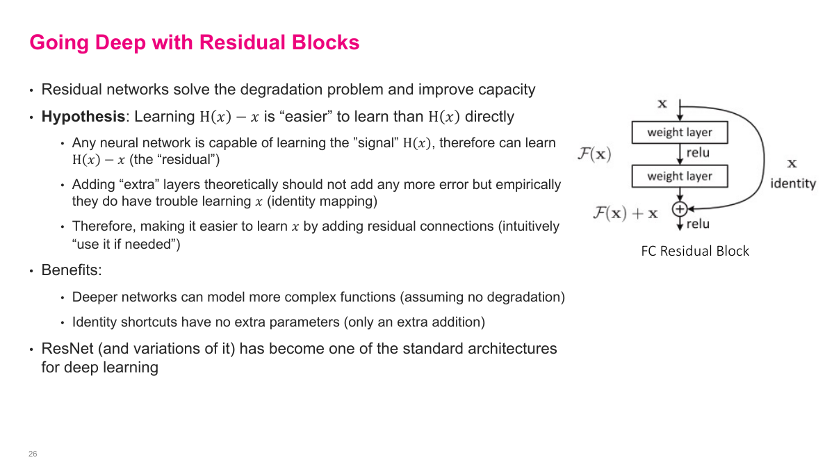
Residual networks introduced an idea that fundamentally changed how we build deep networks. The core problem: as networks get deeper, gradients have to pass through more and more layers during backpropagation, and they tend to vanish or explode. A residual block adds a "shortcut connection" that skips one or more layers -- the input is added directly to the output of the block. So instead of learning a function F(x), the block learns F(x) + x. This means the block only needs to learn the residual -- the difference from the identity. If the optimal transformation is close to the identity (which is common in deep networks), learning a small residual is much easier than learning the full mapping from scratch. This simple change enables training networks with hundreds of layers.

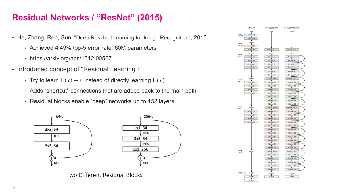
ResNet won ImageNet in 2015 with the lowest error rate at the time. The paper introduced two types of residual blocks: a basic block with two 3x3 convolutions, and a bottleneck block that uses 1x1 convolutions to reduce and then restore depth around a 3x3 convolution. The architecture scales to 50, 101, or even 152 layers. Compared to VGG's 16-19 layers, this was a dramatic increase in depth. ResNet remains one of the most commonly used architectures and is often the default baseline for image classification tasks.

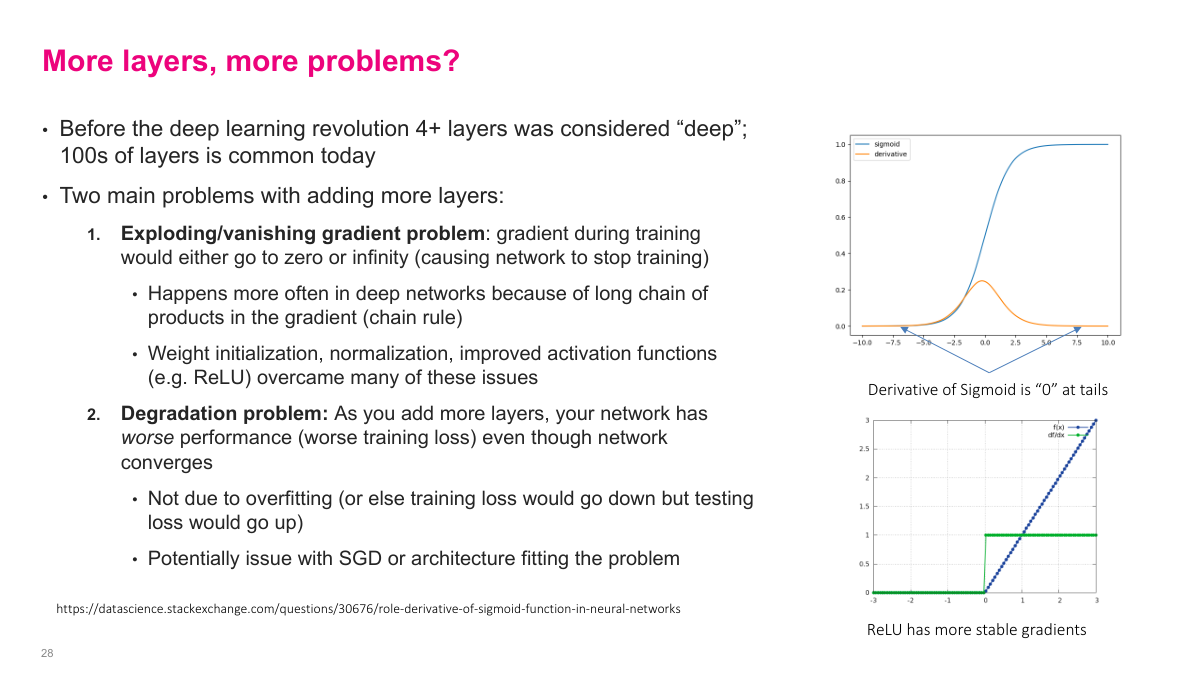
Adding more layers introduces two fundamental problems. First, the exploding/vanishing gradient problem: during backpropagation, the gradient is a product of many intermediate derivatives via the chain rule. If those values are consistently less than one, the gradient vanishes toward zero. If they're greater than one, it explodes. Weight initialization, normalization, and improved activation functions like ReLU (which has a stable gradient of 1 for positive inputs, unlike sigmoid whose derivative approaches zero at the tails) help mitigate this. Second, the degradation problem: as you add more layers, the network actually gets worse training loss -- not because of overfitting, but because the optimization becomes harder. This is what residual connections were designed to solve.

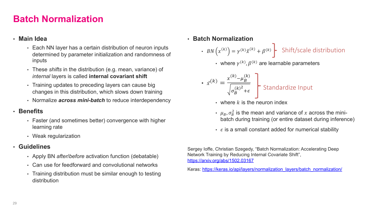
We know that normalizing input data helps training -- if one feature has values in the millions and another is around 0.1, the network struggles. Batch normalization applies this same idea to the internal layers. For each mini-batch, it computes the mean and variance of each feature across all examples in the batch, then normalizes to zero mean and unit variance. After normalizing, it applies learnable scale (gamma) and shift (beta) parameters so the network can undo the normalization if that's optimal. This stabilizes training by ensuring each layer receives inputs with a consistent distribution, regardless of how earlier layers are changing. The result is faster convergence and the ability to use higher learning rates.

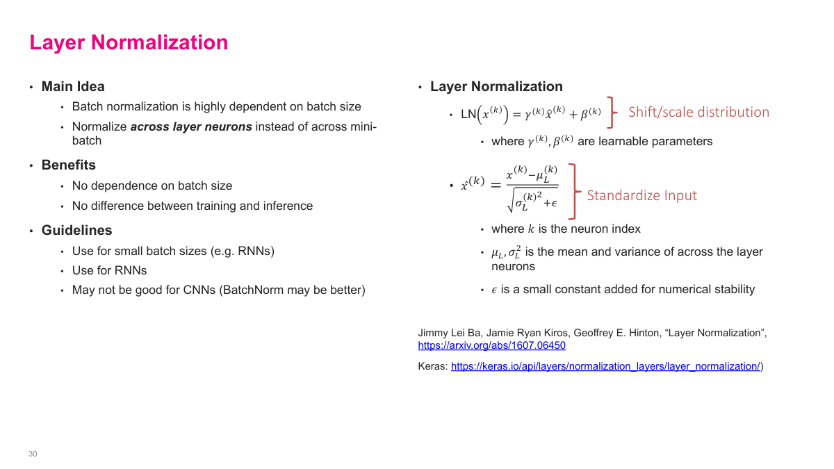
Layer normalization takes a different approach -- instead of normalizing across the batch dimension, it normalizes across the features within a single layer for each example independently. For each input, it computes the mean and variance of all the outputs in that layer, normalizes them, and then applies learnable scale and shift parameters. The advantage over batch normalization is that it doesn't depend on batch size, making it suitable for sequence models and situations where batch statistics are unreliable. You can place either type of normalization after each layer in your network.

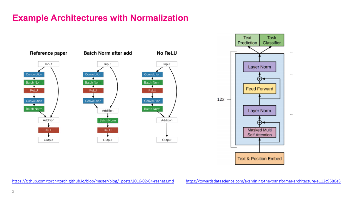
In practice, modern architectures combine all these building blocks. A common CNN pattern is convolution, batch normalization, then ReLU activation -- repeated at each layer. You can place batch norm before or after the activation function; both approaches work. The transformer architecture, shown here on the right, uses layer normalization instead, along with residual connections (the shortcut arrows). In recent papers, you'll see these patterns everywhere: residual connections for gradient flow, normalization layers for training stability, and the two combined enable training very deep networks effectively.

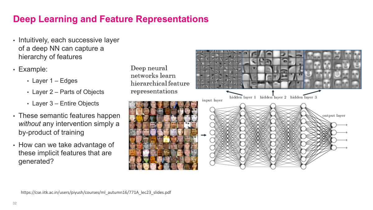
Each successive layer of a deep neural network captures increasingly abstract features. Layer 1 might learn edges, layer 2 learns parts of objects, and layer 3 learns entire objects. This hierarchy emerges automatically from training -- no one tells the network to learn edges first. It's simply a by-product of optimizing the loss function. This observation raises an important question: if a network trained on one task has already learned useful feature representations, can we reuse those features for a different task? That's the motivation for transfer learning.

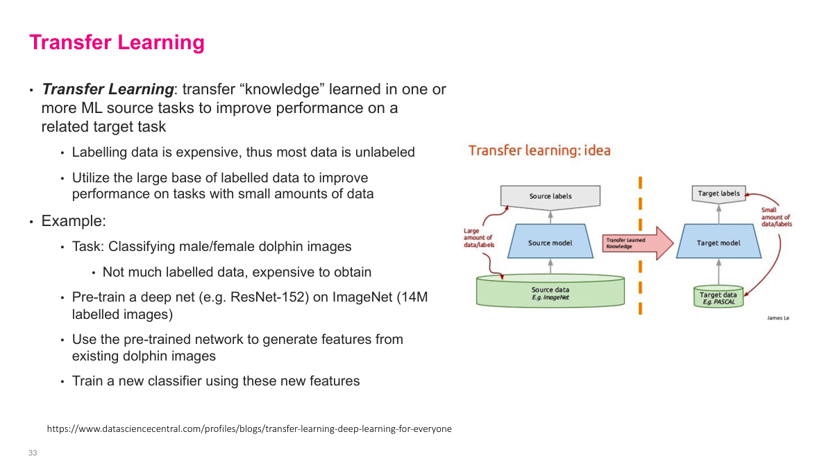
Transfer learning takes a model pre-trained on one task and adapts it for a different task. The idea is that features learned on a large dataset (like ImageNet) are broadly useful -- edges, textures, and object parts transfer well across many vision tasks. Instead of training from scratch, you start with a pre-trained model and either use it as a fixed feature extractor or fine-tune it on your specific dataset. This is especially valuable when you have limited labeled data for your target task, since the pre-trained model already captures useful representations from millions of training examples.

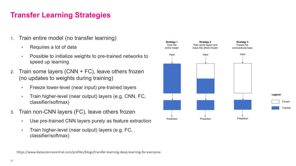
There are three main strategies. First, train the entire model from scratch (no transfer learning) -- this requires a lot of data, though you can still initialize weights from a pre-trained network to speed up learning. Second, freeze the lower-level CNN layers (near the input) and train only the higher-level layers (CNN + FC + classifier) -- this preserves generic features while adapting task-specific ones. Third, freeze all CNN layers entirely and only train the fully connected and classifier layers -- this uses the pre-trained network purely as a feature extractor. Which strategy to use depends on how much data you have and how similar your target task is to the original.

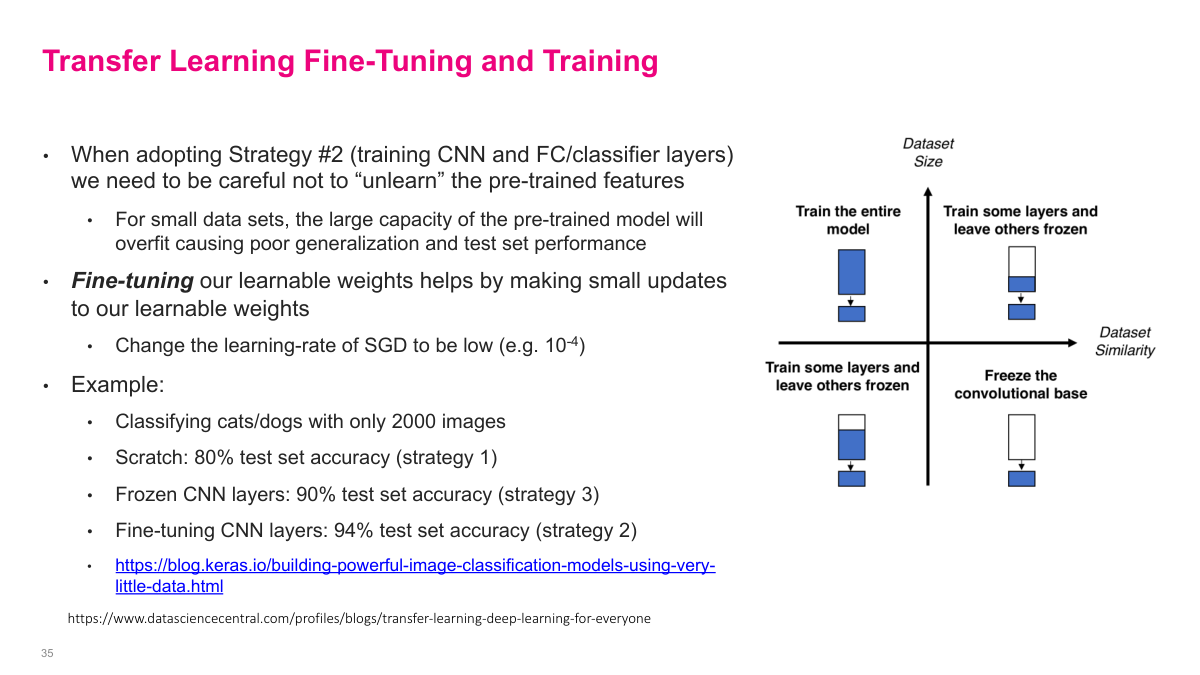
When using Strategy 2 (training some CNN layers), you need to be careful not to "unlearn" the pre-trained features -- with small datasets, the model's large capacity can overfit. Fine-tuning addresses this by using a low learning rate (e.g., 10^-4) to make small weight updates. The results are striking: classifying cats vs. dogs with only 2,000 images, training from scratch achieves 80% accuracy, frozen CNN layers get 90%, and fine-tuning CNN layers reaches 94%. The right strategy also depends on dataset similarity -- a quadrant chart on the slide maps dataset size vs. similarity to recommend which approach to use.

Pre-trained models can be used for transfer learning or directly for the task at hand. Keras provides pre-trained image classification models trained on ImageNet, including ResNet-50, VGG 16/19, and Inception v3. Beyond image classification, many pre-trained models exist for word embeddings trained on large text datasets like Wikipedia and Twitter -- word2Vec (Google), fastText (Facebook), and gensim are popular options. Pre-trained models also exist for object detection, facial recognition, sentiment analysis, segmentation, and image/text generation. You can get state-of-the-art results without training a single neuron.